Third eye • StrategyThird eye • Strategy – User Guide
1. Idea & Concept
Third eye • Strategy combines three things into one system:
Ichimoku Cloud – to define market regime and support/resistance.
Moving Average (trend filter) – to trade only in the dominant direction.
CCI (Commodity Channel Index) – to generate precise entry signals on momentum breakouts.
The script is a strategy, not an indicator: it can backtest entries, exits, SL, TP and BreakEven logic automatically.
2. Indicators Used
2.1 Ichimoku
Standard Ichimoku settings (by default 9/26/52/26) are used:
Conversion Line (Tenkan-sen)
Base Line (Kijun-sen)
Leading Span A & B (Kumo Cloud)
Lagging Span is calculated but hidden from the chart (for visual simplicity).
From the cloud we derive:
kumoTop – top of the cloud under current price.
kumoBottom – bottom of the cloud under current price.
Flags:
is_above_kumo – price above the cloud.
is_below_kumo – price below the cloud.
is_in_kumo – price inside the cloud.
These conditions are used as trend / regime filters and for stop-loss & trailing stops.
2.2 Moving Average
You can optionally display and use a trend MA:
Types: SMA, EMA, DEMA, WMA
Length: configurable (default 200)
Source: default close
Filter idea:
If MA Direction Filter is ON:
When Close > MA → strategy allows only Long signals.
When Close < MA → strategy allows only Short signals.
The MA is plotted on the chart (if enabled).
2.3 CCI & Panel
The CCI (Commodity Channel Index) is used for entry timing:
CCI length and source are configurable (default length 20, source hlc3).
Two thresholds:
CCI Upper Threshold (Long) – default +100
CCI Lower Threshold (Short) – default –100
Signals:
Long signal:
CCI crosses up through the upper threshold
cci_val < upper_threshold and cci_val > upper_threshold
Short signal:
CCI crosses down through the lower threshold
cci_val > lower_threshold and cci_val < lower_threshold
There is a panel (table) in the bottom-right corner:
Shows current CCI value.
Shows filter status as colored dots:
Green = filter enabled and passed.
Red = filter enabled and blocking trades.
Gray = filter is disabled.
Filters shown in the panel:
Ichimoku Cloud filter (Long/Short)
Ichimoku Lines filter (Conversion/Base vs Cloud)
MA Direction filter
3. Filters & Trade Direction
All filters can be turned ON/OFF independently.
3.1 Ichimoku Cloud Filter
Purpose: trade only when price is clearly above or below the Kumo.
Long Cloud Filter (Use Ichimoku Cloud Filter) – when enabled:
Long trades only if close > cloud top.
Short Cloud Filter – when enabled:
Short trades only if close < cloud bottom.
If the cloud filter is disabled, this condition is ignored.
3.2 Ichimoku Lines Above/Below Cloud
Purpose: stronger trend confirmation: Ichimoku lines should also be on the “correct” side of the cloud.
Long Lines Filter:
Long allowed only if Conversion Line and Base Line are both above the cloud.
Short Lines Filter:
Short allowed only if both lines are below the cloud.
If this filter is OFF, the conditions are not checked.
3.3 MA Direction Filter
As described above:
When ON:
Close > MA → only Longs.
Close < MA → only Shorts.
4. Anti-Re-Entry Logic (Cloud Touch Reset)
The strategy uses internal flags to avoid continuous re-entries in the same direction without a reset.
Two flags:
allowLong
allowShort
After a Long entry, allowLong is set to false, allowShort to true.
After a Short entry, allowShort is set to false, allowLong to true.
Flags are reset when price touches the Kumo:
If Low goes into the cloud → allowLong = true
If High goes into the cloud → allowShort = true
If Close is inside the cloud → both allowLong and allowShort are set to true
There is a key option:
Wait Position Close Before Flag Reset
If ON: cloud touch will reset flags only when there is no open position.
If OFF: flags can be reset even while a trade is open.
This gives a kind of regime-based re-entry control: after a trend leg, you wait for a “cloud interaction” to allow new signals.
5. Risk Management
All risk management is handled inside the strategy.
5.1 Position Sizing
Order Size % of Equity – default 10%
The strategy calculates:
position_value = equity * (Order Size % / 100)
position_qty = position_value / close
So position size automatically adapts to your current equity.
5.2 Take Profit Modes
You can choose one of two TP modes:
Percent
Fibonacci
5.2.1 Percent Mode
Single Take Profit at X% from entry (default 2%).
For Long:
TP = entry_price * (1 + tp_pct / 100)
For Short:
TP = entry_price * (1 - tp_pct / 100)
One strategy.exit per side is used: "Long TP/SL" and "Short TP/SL".
5.2.2 Fibonacci Mode (2 partial TPs)
In this mode, TP levels are based on a virtual Fib-style extension between entry and stop-loss.
Inputs:
Fib TP1 Level (default 1.618)
Fib TP2 Level (default 2.5)
TP1 Share % (Fib) (default 50%)
TP2 share is automatically 100% - TP1 share.
Process for Long:
Compute a reference Stop (see SL section below) → sl_for_fib.
Compute distance: dist = entry_price - sl_for_fib.
TP levels:
TP1 = entry_price + dist * (Fib TP1 Level - 1)
TP2 = entry_price + dist * (Fib TP2 Level - 1)
For Short, the logic is mirrored.
Two exits are used:
TP1 – closes TP1 share % of position.
TP2 – closes remaining TP2 share %.
Same stop is used for both partial exits.
5.3 Stop-Loss Modes
You can choose one of three Stop Loss modes:
Stable – fixed % from entry.
Ichimoku – fixed level derived from the Kumo.
Ichimoku Trailing – dynamic SL following the cloud.
5.3.1 Stable SL
For Long:
SL = entry_price * (1 - Stable SL % / 100)
For Short:
SL = entry_price * (1 + Stable SL % / 100)
Used both for Percent TP mode and as reference for Fib TP if Kumo is not available.
5.3.2 Ichimoku SL (fixed, non-trailing)
At the time of a new trade:
For Long:
Base SL = cloud bottom minus small offset (%)
For Short:
Base SL = cloud top plus small offset (%)
The offset is configurable: Ichimoku SL Offset %.
Once computed, that SL level is fixed for this trade.
5.3.3 Ichimoku Trailing SL
Similar to Ichimoku SL, but recomputed each bar:
For Long:
SL = cloud bottom – offset
For Short:
SL = cloud top + offset
A red trailing SL line is drawn on the chart to visualize current stop level.
This trailing SL is also used as reference for BreakEven and for Fib TP distance.
6. BreakEven Logic (with BE Lines)
BreakEven is optional and supports two modes:
Percent
Fibonacci
Inputs:
Percent mode:
BE Trigger % (from entry) – move SL to BE when price goes this % in profit.
BE Offset % from entry – SL will be set to entry ± this offset.
Fibonacci mode:
BE Fib Level – Fib level at which BE will be activated (default 1.618, same style as TP).
BE Offset % from entry – how far from entry to place BE stop.
The logic:
Before BE is triggered, SL follows its normal mode (Stable/Ichimoku/Ichimoku Trailing).
When BE triggers:
For Long:
New SL = max(current SL, BE SL).
For Short:
New SL = min(current SL, BE SL).
This means BE will never loosen the stop – only tighten it.
When BE is activated, the strategy draws a violet horizontal line at the BreakEven level (once per trade).
BE state is cleared when the position is closed or when a new position is opened.
7. Entry & Exit Logic (Summary)
7.1 Long Entry
Conditions for a Long:
CCI signal:
CCI crosses up through the upper threshold.
Ichimoku Cloud Filter (optional):
If enabled → price must be above the Kumo.
Ichimoku Lines Filter (optional):
If enabled → Conversion Line and Base Line must be above the Kumo.
MA Direction Filter (optional):
If enabled → Close must be above the chosen MA.
Anti-re-entry flag:
allowLong must be true (cloud-based reset).
Position check:
Long entries are allowed when current position size ≤ 0 (so it can also reverse from short to long).
If all these conditions are true, the strategy sends:
strategy.entry("Long", strategy.long, qty = calculated_qty)
After entry:
allowLong = false
allowShort = true
7.2 Short Entry
Same structure, mirrored:
CCI signal:
CCI crosses down through the lower threshold.
Cloud filter: price must be below cloud (if enabled).
Lines filter: conversion & base must be below cloud (if enabled).
MA filter: Close must be below MA (if enabled).
allowShort must be true.
Position check: position size ≥ 0 (allows reversal from long to short).
Then:
strategy.entry("Short", strategy.short, qty = calculated_qty)
Flags update:
allowShort = false
allowLong = true
7.3 Exits
While in a position:
The strategy continuously recalculates SL (depending on chosen mode) and, in Percent mode, TP.
In Fib mode, fixed TP levels are computed at entry.
BreakEven may raise/tighten the SL if its conditions are met.
Exits are executed via strategy.exit:
Percent mode: one TP+SL exit per side.
Fib mode: two partial exits (TP1 and TP2) sharing the same SL.
At position open, the script also draws visual lines:
White line — entry price.
Green line(s) — TP level(s).
Red line — SL (if not using Ichimoku Trailing; with trailing, the red line is updated dynamically).
Maximum of 30 lines are kept to avoid clutter.
8. How to Use the Strategy
Choose market & timeframe
Works well on trending instruments. Try crypto, FX or indices on H1–H4, or intraday if you prefer more trades.
Adjust Ichimoku settings
Keep defaults (9/26/52/26) or adapt to your timeframe.
Configure Moving Average
Typical: EMA 200 as a trend filter.
Turn MA Direction Filter ON if you want to trade only with the main trend.
Set CCI thresholds
Default ±100 is classic.
Lower thresholds → more signals, higher noise.
Higher thresholds → fewer but stronger signals.
Enable/disable filters
Turn on Ichimoku Cloud and Ichimoku Lines if you want only “clean” trend trades.
Use Wait Position Close Before Flag Reset to control how often re-entries are allowed.
Choose TP & SL mode
Percent mode is simpler and easier to understand.
Fibonacci mode is more advanced: it aligns TP levels with the distance to stop, giving asymmetric RR setups (two partial TPs).
Choose Stable SL for fixed-risk trades, or Ichimoku / Ichimoku Trailing to tie stops to the cloud structure.
Set BreakEven
Enable BE if you want to lock in risk-free trades after a certain move.
Percent mode is straightforward; Fib mode keeps BreakEven in harmony with your Fib TP setup.
Run Backtest & Optimize
Press “Add to chart” → go to Strategy Tester.
Adjust parameters to your market and timeframe.
Look at equity curve, PF, drawdown, average trade, etc.
Live / Paper Trading
After you’re satisfied with backtest results, use the strategy to generate signals.
You can mirror entries/exits manually or connect them to alerts (if you build an alert-based execution layer).
Cari dalam skrip untuk "the strat"

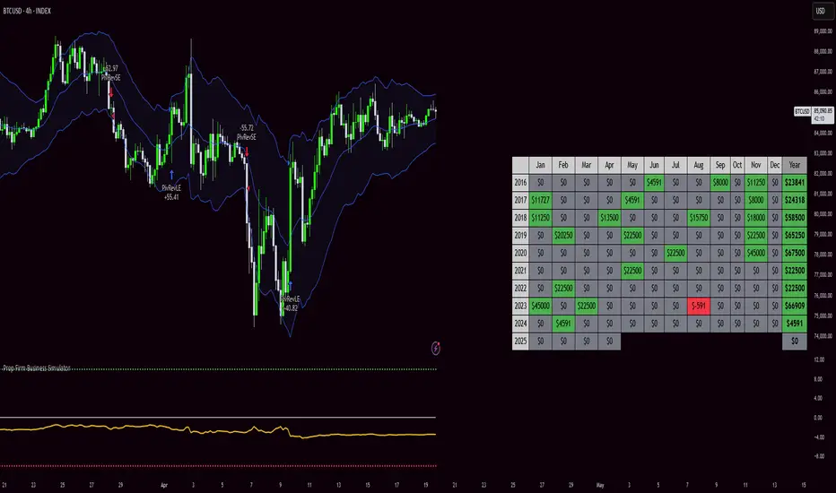
Prop Firm Business SimulatorThe prop firm business simulator is exactly what it sounds like. It's a plug and play tool to test out any tradingview strategy and simulate hypothetical performance on CFD Prop Firms.
Now what is a modern day CFD Prop Firm?
These companies sell simulated trading challenges for a challenge fee. If you complete the challenge you get access to simulated capital and you get a portion of the profits you make on those accounts payed out.
I've included some popular firms in the code as presets so it's easy to simulate them. Take into account that this info will likely be out of date soon as these prices and challenge conditions change.
Also, this tool will never be able to 100% simulate prop firm conditions and all their rules. All I aim to do with this tool is provide estimations.
Now why is this tool helpful?
Most traders on here want to turn their passion into their full-time career, prop firms have lately been the buzz in the trading community and market themselves as a faster way to reach that goal.
While this all sounds great on paper, it is sometimes hard to estimate how much money you will have to burn on challenge fees and set realistic monthly payout expectations for yourself and your trading. This is where this tool comes in.
I've specifically developed this for traders that want to treat prop firms as a business. And as a business you want to know your monthly costs and income depending on the trading strategy and prop firm challenge you are using.
How to use this tool
It's quite simple you remove the top part of the script and replace it with your own strategy. Make sure it's written in same version of pinescript before you do that.
//--$$$$$$$$$$$$$$$$$$$$$$$$$$$$$$$$$$$$$$$$$$$$$$$$--//--------------------------------------------------------------------------------------------------------------------------$$$$$$
//--$$$$$--Strategy-- --$$$$$$--// ******************************************************************************************************************************
//--$$$$$$$$$$$$$$$$$$$$$$$$$$$$$$$$$$$$$$$$$$$$$$$$--//--------------------------------------------------------------------------------------------------------------------------$$$$$$
length = input.int(20, minval=1, group="Keltner Channel Breakout")
mult = input(2.0, "Multiplier", group="Keltner Channel Breakout")
src = input(close, title="Source", group="Keltner Channel Breakout")
exp = input(true, "Use Exponential MA", display = display.data_window, group="Keltner Channel Breakout")
BandsStyle = input.string("Average True Range", options = , title="Bands Style", display = display.data_window, group="Keltner Channel Breakout")
atrlength = input(10, "ATR Length", display = display.data_window, group="Keltner Channel Breakout")
esma(source, length)=>
s = ta.sma(source, length)
e = ta.ema(source, length)
exp ? e : s
ma = esma(src, length)
rangema = BandsStyle == "True Range" ? ta.tr(true) : BandsStyle == "Average True Range" ? ta.atr(atrlength) : ta.rma(high - low, length)
upper = ma + rangema * mult
lower = ma - rangema * mult
//--Graphical Display--// *-*-*-*-*-*-*-*-*-*-*-*-*-*-*-*-*-*-*-*-*-*-*-*-*-*-*-*-*-*-*-*-*-*-*-*-*-*-*-*-*-*-*-*-*-*-*-*-*-*-*-*-*-*-*-*-*-*-*-*-*-*-*-*-*-*-*-*-*-*-*-*-*-$$$$$$
u = plot(upper, color=#2962FF, title="Upper", force_overlay=true)
plot(ma, color=#2962FF, title="Basis", force_overlay=true)
l = plot(lower, color=#2962FF, title="Lower", force_overlay=true)
fill(u, l, color=color.rgb(33, 150, 243, 95), title="Background")
//--Risk Management--// *-*-*-*-*-*-*-*-*-*-*-*-*-*-*-*-*-*-*-*-*-*-*-*-*-*-*-*-*-*-*-*-*-*-*-*-*-*-*-*-*-*-*-*-*-*-*-*-*-*-*-*-*-*-*-*-*-*-*-*-*-*-*-*-*-*-*-*-*-*-*-*-*-*-$$$$$$
riskPerTradePerc = input.float(1, title="Risk per trade (%)", group="Keltner Channel Breakout")
le = high>upper ? false : true
se = lowlower
strategy.entry('PivRevLE', strategy.long, comment = 'PivRevLE', stop = upper, qty=riskToLots)
if se and upper>lower
strategy.entry('PivRevSE', strategy.short, comment = 'PivRevSE', stop = lower, qty=riskToLots)
The tool will then use the strategy equity of your own strategy and use this to simulat prop firms. Since these CFD prop firms work with different phases and payouts the indicator will simulate the gains until target or max drawdown / daily drawdown limit gets reached. If it reaches target it will go to the next phase and keep on doing that until it fails a challenge.
If in one of the phases there is a reward for completing, like a payout, refund, extra it will add this to the gains.
If you fail the challenge by reaching max drawdown or daily drawdown limit it will substract the challenge fee from the gains.
These gains are then visualised in the calendar so you can get an idea of yearly / monthly gains of the backtest. Remember, it is just a backtest so no guarantees of future income.
The bottom pane (non-overlay) is visualising the performance of the backtest during the phases. This way u can check if it is realistic. For instance if it only takes 1 bar on chart to reach target you are probably risking more than the firm wants you to risk. Also, it becomes much less clear if daily drawdown got hit in those high risk strategies, the results will be less accurate.
The daily drawdown limit get's reset every time there is a new dayofweek on chart.
If you set your prop firm preset setting to "'custom" the settings below that are applied as your prop firm settings. Otherwise it will use one of the template by default it's FTMO 100K.
The strategy I'm using as an example in this script is a simple Keltner Channel breakout strategy. I'm using a 0.05% commission per trade as that is what I found most common on crypto exchanges and it's close to the commissions+spread you get on a cfd prop firm. I'm targeting a 1% risk per trade in the backtest to try and stay within prop firm boundaries of max 1% risk per trade.
Lastly, the original yearly and monthly performance table was developed by Quantnomad and I've build ontop of that code. Here's a link to the original publication:
That's everything for now, hope this indicator helps people visualise the potential of prop firms better or to understand that they are not a good fit for their current financial situation.
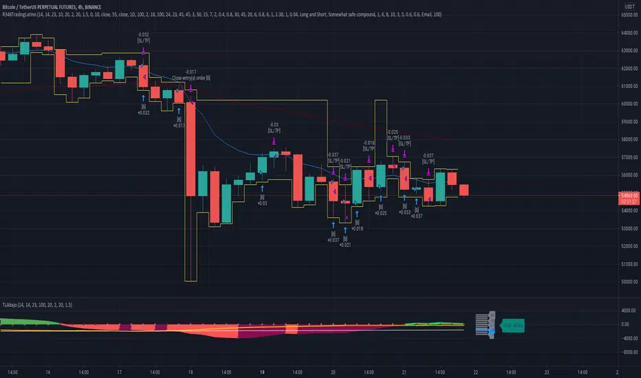
Ruckard TradingLatinoThis strategy tries to mimic TradingLatino strategy.
The current implementation is beta.
Si hablas castellano o espanyol por favor consulta MENSAJE EN CASTELLANO más abajo.
It's aimed at BTCUSDT pair and 4h timeframe.
STRATEGY DEFAULT SETTINGS EXPLANATION
max_bars_back=5000 : This is a random number of bars so that the strategy test lasts for one or two years
calc_on_order_fills=false : To wait for the 4h closing is too much. Try to check if it's worth entering a position after closing one. I finally decided not to recheck if it's worth entering after an order is closed. So it is false.
calc_on_every_tick=false
pyramiding=0 : We only want one entry allowed in the same direction. And we don't want the order to scale by error.
initial_capital=1000 : These are 1000 USDT. By using 1% maximum loss per trade and 7% as a default stop loss by using 1000 USDT at 12000 USDT per BTC price you would entry with around 142 USDT which are converted into: 0.010 BTC . The maximum number of decimal for contracts on this BTCUSDT market is 3 decimals. E.g. the minimum might be: 0.001 BTC . So, this minimal 1000 amount ensures us not to entry with less than 0.001 entries which might have happened when using 100 USDT as an initial capital.
slippage=1 : Binance BTCUSDT mintick is: 0.01. Binance slippage: 0.1 % (Let's assume). TV has an integer slippage. It does not have a percentage based slippage. If we assume a 1000 initial capital, the recommended equity is 142 which at 11996 USDT per BTC price means: 0.011 BTC. The 0.1% slippage of: 0.011 BTC would be: 0.000011 . This is way smaller than the mintick. So our slippage is going to be 1. E.g. 1 (slippage) * 0.01 (mintick)
commission_type=strategy.commission.percent and commission_value=0.1 : According to: binance . com / en / fee / schedule in VIP 0 level both maker and taker fees are: 0.1 %.
BACKGROUND
Jaime Merino is a well known Youtuber focused on crypto trading
His channel TradingLatino
features monday to friday videos where he explains his strategy.
JAIME MERINO STANCE ON BOTS
Jaime Merino stance on bots (taken from memory out of a 2020 June video from him):
'~
You know. They can program you a bot and it might work.
But, there are some special situations that the bot would not be able to handle.
And, I, as a human, I would handle it. And the bot wouldn't do it.
~'
My long term target with this strategy script is add as many
special situations as I can to the script
so that it can match Jaime Merino behaviour even in non normal circumstances.
My alternate target is learn Pine script
and enjoy programming with it.
WARNING
This script might be bigger than other TradingView scripts.
However, please, do not be confused because the current status is beta.
This script has not been tested with real money.
This is NOT an official strategy from Jaime Merino.
This is NOT an official strategy from TradingLatino . net .
HOW IT WORKS
It basically uses ADX slope and LazyBear's Squeeze Momentum Indicator
to make its buy and sell decisions.
Fast paced EMA being bigger than slow paced EMA
(on higher timeframe) advices going long.
Fast paced EMA being smaller than slow paced EMA
(on higher timeframe) advices going short.
It finally add many substrats that TradingLatino uses.
SETTINGS
__ SETTINGS - Basics
____ SETTINGS - Basics - ADX
(ADX) Smoothing {14}
(ADX) DI Length {14}
(ADX) key level {23}
____ SETTINGS - Basics - LazyBear Squeeze Momentum
(SQZMOM) BB Length {20}
(SQZMOM) BB MultFactor {2.0}
(SQZMOM) KC Length {20}
(SQZMOM) KC MultFactor {1.5}
(SQZMOM) Use TrueRange (KC) {True}
____ SETTINGS - Basics - EMAs
(EMAS) EMA10 - Length {10}
(EMAS) EMA10 - Source {close}
(EMAS) EMA55 - Length {55}
(EMAS) EMA55 - Source {close}
____ SETTINGS - Volume Profile
Lowest and highest VPoC from last three days
is used to know if an entry has a support
VPVR of last 100 4h bars
is also taken into account
(VP) Use number of bars (not VP timeframe): Uses 'Number of bars {100}' setting instead of 'Volume Profile timeframe' setting for calculating session VPoC
(VP) Show tick difference from current price {False}: BETA . Might be useful for actions some day.
(VP) Number of bars {100}: If 'Use number of bars (not VP timeframe)' is turned on this setting is used to calculate session VPoC.
(VP) Volume Profile timeframe {1 day}: If 'Use number of bars (not VP timeframe)' is turned off this setting is used to calculate session VPoC.
(VP) Row width multiplier {0.6}: Adjust how the extra Volume Profile bars are shown in the chart.
(VP) Resistances prices number of decimal digits : Round Volume Profile bars label numbers so that they don't have so many decimals.
(VP) Number of bars for bottom VPOC {18}: 18 bars equals 3 days in suggested timeframe of 4 hours. It's used to calculate lowest session VPoC from previous three days. It's also used as a top VPOC for sells.
(VP) Ignore VPOC bottom advice on long {False}: If turned on it ignores bottom VPOC (or top VPOC on sells) when evaluating if a buy entry is worth it.
(VP) Number of bars for VPVR VPOC {100}: Number of bars to calculate the VPVR VPoC. We use 100 as Jaime once used. When the price bounces back to the EMA55 it might just bounce to this VPVR VPoC if its price it's lower than the EMA55 (Sells have inverse algorithm).
____ SETTINGS - ADX Slope
ADX Slope
help us to understand if ADX
has a positive slope, negative slope
or it is rather still.
(ADXSLOPE) ADX cut {23}: If ADX value is greater than this cut (23) then ADX has strength
(ADXSLOPE) ADX minimum steepness entry {45}: ADX slope needs to be 45 degrees to be considered as a positive one.
(ADXSLOPE) ADX minimum steepness exit {45}: ADX slope needs to be -45 degrees to be considered as a negative one.
(ADXSLOPE) ADX steepness periods {3}: In order to avoid false detection the slope is calculated along 3 periods.
____ SETTINGS - Next to EMA55
(NEXTEMA55) EMA10 to EMA55 bounce back percentage {80}: EMA10 might bounce back to EMA55 or maybe to 80% of its complete way to EMA55
(NEXTEMA55) Next to EMA55 percentage {15}: How much next to the EMA55 you need to be to consider it's going to bounce back upwards again.
____ SETTINGS - Stop Loss and Take Profit
You can set a default stop loss or a default take profit.
(STOPTAKE) Stop Loss % {7.0}
(STOPTAKE) Take Profit % {2.0}
____ SETTINGS - Trailing Take Profit
You can customize the default trailing take profit values
(TRAILING) Trailing Take Profit (%) {1.0}: Trailing take profit offset in percentage
(TRAILING) Trailing Take Profit Trigger (%) {2.0}: When 2.0% of benefit is reached then activate the trailing take profit.
____ SETTINGS - MAIN TURN ON/OFF OPTIONS
(EMAS) Ignore advice based on emas {false}.
(EMAS) Ignore advice based on emas (On closing long signal) {False}: Ignore advice based on emas but only when deciding to close a buy entry.
(SQZMOM) Ignore advice based on SQZMOM {false}: Ignores advice based on SQZMOM indicator.
(ADXSLOPE) Ignore advice based on ADX positive slope {false}
(ADXSLOPE) Ignore advice based on ADX cut (23) {true}
(STOPTAKE) Take Profit? {false}: Enables simple Take Profit.
(STOPTAKE) Stop Loss? {True}: Enables simple Stop Loss.
(TRAILING) Enable Trailing Take Profit (%) {True}: Enables Trailing Take Profit.
____ SETTINGS - Strategy mode
(STRAT) Type Strategy: 'Long and Short', 'Long Only' or 'Short Only'. Default: 'Long and Short'.
____ SETTINGS - Risk Management
(RISKM) Risk Management Type: 'Safe', 'Somewhat safe compound' or 'Unsafe compound'. ' Safe ': Calculations are always done with the initial capital (1000) in mind. The maximum losses per trade/day/week/month are taken into account. ' Somewhat safe compound ': Calculations are done with initial capital (1000) or a higher capital if it increases. The maximum losses per trade/day/week/month are taken into account. ' Unsafe compound ': In each order all the current capital is gambled and only the default stop loss per order is taken into account. That means that the maximum losses per trade/day/week/month are not taken into account. Default : 'Somewhat safe compound'.
(RISKM) Maximum loss per trade % {1.0}.
(RISKM) Maximum loss per day % {6.0}.
(RISKM) Maximum loss per week % {8.0}.
(RISKM) Maximum loss per month % {10.0}.
____ SETTINGS - Decimals
(DECIMAL) Maximum number of decimal for contracts {3}: How small (3 decimals means 0.001) an entry position might be in your exchange.
EXTRA 1 - PRICE IS IN RANGE indicator
(PRANGE) Print price is in range {False}: Enable a bottom label that indicates if the price is in range or not.
(PRANGE) Price range periods {5}: How many previous periods are used to calculate the medians
(PRANGE) Price range maximum desviation (%) {0.6} ( > 0 ): Maximum positive desviation for range detection
(PRANGE) Price range minimum desviation (%) {0.6} ( > 0 ): Mininum negative desviation for range detection
EXTRA 2 - SQUEEZE MOMENTUM Desviation indicator
(SQZDIVER) Show degrees {False}: Show degrees of each Squeeze Momentum Divergence lines to the x-axis.
(SQZDIVER) Show desviation labels {False}: Whether to show or not desviation labels for the Squeeze Momentum Divergences.
(SQZDIVER) Show desviation lines {False}: Whether to show or not desviation lines for the Squeeze Momentum Divergences.
EXTRA 3 - VOLUME PROFILE indicator
WARNING: This indicator works not on current bar but on previous bar. So in the worst case it might be VP from 4 hours ago. Don't worry, inside the strategy calculus the correct values are used. It's just that I cannot show the most recent one in the chart.
(VP) Print recent profile {False}: Show Volume Profile indicator
(VP) Avoid label price overlaps {False}: Avoid label prices to overlap on the chart.
EXTRA 4 - ZIGNALY SUPPORT
(ZIG) Zignaly Alert Type {Email}: 'Email', 'Webhook'. ' Email ': Prepare alert_message variable content to be compatible with zignaly expected email content format. ' Webhook ': Prepare alert_message variable content to be compatible with zignaly expected json content format.
EXTRA 5 - DEBUG
(DEBUG) Enable debug on order comments {False}: If set to true it prepares the order message to match the alert_message variable. It makes easier to debug what would have been sent by email or webhook on each of the times an order is triggered.
HOW TO USE THIS STRATEGY
BOT MODE: This is the default setting.
PROPER VOLUME PROFILE VIEWING: Click on this strategy settings. Properties tab. Make sure Recalculate 'each time the order was run' is turned off.
NEWBIE USER: (Check PROPER VOLUME PROFILE VIEWING above!) You might want to turn on the 'Print recent profile {False}' setting. Alternatively you can use my alternate realtime study: 'Resistances and supports based on simplified Volume Profile' but, be aware, it might consume one indicator.
ADVANCED USER 1: Turn on the 'Print price is in range {False}' setting and help us to debug this subindicator. Also help us to figure out how to include this value in the strategy.
ADVANCED USER 2: Turn on the all the (SQZDIVER) settings and help us to figure out how to include this value in the strategy.
ADVANCED USER 3: (Check PROPER VOLUME PROFILE VIEWING above!) Turn on the 'Print recent profile {False}' setting and report any problem with it.
JAIME MERINO: Just use the indicator as it comes by default. It should only show BUY signals, SELL signals and their associated closing signals. From time to time you might want to check 'ADVANCED USER 2' instructions to check that there's actually a divergence. Check also 'ADVANCED USER 1' instructions for your amusement.
EXTRA ADVICE
It's advised that you use this strategy in addition to these two other indicators:
* Squeeze Momentum Indicator
* ADX
so that your chart matches as close as possible to TradingLatino chart.
ZIGNALY INTEGRATION
This strategy supports Zignaly email integration by default. It also supports Zignaly Webhook integration.
ZIGNALY INTEGRATION - Email integration example
What you would write in your alert message:
||{{strategy.order.alert_message}}||key=MYSECRETKEY||
ZIGNALY INTEGRATION - Webhook integration example
What you would write in your alert message:
{ {{strategy.order.alert_message}} , "key" : "MYSECRETKEY" }
CREDITS
I have reused and adapted some code from
'Directional Movement Index + ADX & Keylevel Support' study
which it's from TradingView console user.
I have reused and adapted some code from
'3ema' study
which it's from TradingView hunganhnguyen1193 user.
I have reused and adapted some code from
'Squeeze Momentum Indicator ' study
which it's from TradingView LazyBear user.
I have reused and adapted some code from
'Strategy Tester EMA-SMA-RSI-MACD' study
which it's from TradingView fikira user.
I have reused and adapted some code from
'Support Resistance MTF' study
which it's from TradingView LonesomeTheBlue user.
I have reused and adapted some code from
'TF Segmented Linear Regression' study
which it's from TradingView alexgrover user.
I have reused and adapted some code from
"Poor man's volume profile" study
which it's from TradingView IldarAkhmetgaleev user.
FEEDBACK
Please check the strategy source code for more detailed information
where, among others, I explain all of the substrats
and if they are implemented or not.
Q1. Did I understand wrong any of the Jaime substrats (which I have implemented)?
Q2. The strategy yields quite profit when we should long (EMA10 from 1d timeframe is higher than EMA55 from 1d timeframe.
Why the strategy yields much less profit when we should short (EMA10 from 1d timeframe is lower than EMA55 from 1d timeframe)?
Any idea if you need to do something else rather than just reverse what Jaime does when longing?
FREQUENTLY ASKED QUESTIONS
FAQ1. Why are you giving this strategy for free?
TradingLatino and his fellow enthusiasts taught me this strategy. Now I'm giving back to them.
FAQ2. Seriously! Why are you giving this strategy for free?
I'm confident his strategy might be improved a lot. By keeping it to myself I would avoid other people contributions to improve it.
Now that everyone can contribute this is a win-win.
FAQ3. How can I connect this strategy to my Exchange account?
It seems that you can attach alerts to strategies.
You might want to combine it with a paying account which enable Webhook URLs to work.
I don't know how all of this works right now so I cannot give you advice on it.
You will have to do your own research on this subject. But, be careful. Automating trades, if not done properly,
might end on you automating losses.
FAQ4. I have just found that this strategy by default gives more than 3.97% of 'maximum series of losses'. That's unacceptable according to my risk management policy.
You might want to reduce default stop loss setting from 7% to something like 5% till you are ok with the 'maximum series of losses'.
FAQ5. Where can I learn more about your work on this strategy?
Check the source code. You might find unused strategies. Either because there's not a substantial increases on earnings. Or maybe because they have not been implemented yet.
FAQ6. How much leverage is applied in this strategy?
No leverage.
FAQ7. Any difference with original Jaime Merino strategy?
Most of the times Jaime defines an stop loss at the price entry. That's not the case here. The default stop loss is 7% (but, don't be confused it only means losing 1% of your investment thanks to risk management). There's also a trailing take profit that triggers at 2% profit with a 1% trailing.
FAQ8. Why this strategy return is so small?
The strategy should be improved a lot. And, well, backtesting in this platform is not guaranteed to return theoric results comparable to real-life returns. That's why I'm personally forward testing this strategy to verify it.
MENSAJE EN CASTELLANO
En primer lugar se agradece feedback para mejorar la estrategia.
Si eres un usuario avanzado y quieres colaborar en mejorar el script no dudes en comentar abajo.
Ten en cuenta que aunque toda esta descripción tenga que estar en inglés no es obligatorio que el comentario esté en inglés.
CHISTE - CASTELLANO
¡Pero Jaime!
¡400.000!
¡Tu da mun!
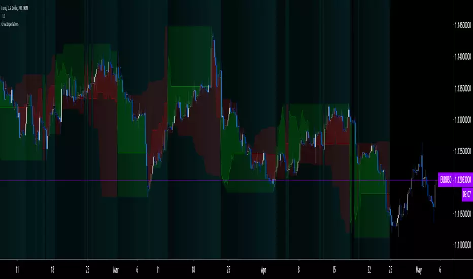
Great Expectations [LucF]Great Expectations helps traders answer the question: What is possible? It is a powerful question, yet exploration of the unknown always entails risk. A more complete set of questions better suited to traders could be:
What opportunity exists from any given point on a chart?
What portion of this opportunity can be realistically captured?
What risk will be incurred in trying to do so, and how long will it take?
Great Expectations is the result of an exploration of these questions. It is a trade simulator that generates visual and quantitative information to help strategy modelers visually identify and analyse areas of optimal expectation on charts, whether they are designing automated or discretionary strategies.
WARNING: Great Expectations is NOT an indicator that helps determine the current state of a market. It works by looking at points in the past from which the future is already known. It uses one definition of repainting extensively (i.e. it goes back in the past to print information that could not have been know at the time). Repainting understood that way is in fact almost all the indicator does! —albeit for what I hope is a noble cause. The indicator is of no use whatsoever in analyzing markets in real-time. If you do not understand what it does, please stay away!
This is an indicator—not a strategy that uses TradingView’s backtesting engine. It works by simulating trades, not unlike a backtest, but with the crucial difference that it assumes a trade (either long or short) is entered on all bars in the historic sample. It walks forward from each bar and determines possible outcomes, gathering individual trade statistics that in turn generate precious global statistics from all outcomes tested on the chart.
Great Expectations provides numbers summarizing trade results on all simulations run from the chart. Those numbers cannot be compared to backtest-produced numbers since all non-filtered bars are examined, even if an entry was taken on the bar immediately preceding the current one, which never happens in a backtest. This peculiarity does NOT invalidate Great Expectations calculations; it just entails that results be considered under a different light. Provided they are evaluated within the indicator’s context, they can be useful—sometimes even more than backtesting results, e.g. in evaluating the impact of parameter-fitting or variations in entry, exit or filtering strats.
Traders and strategy modelers are creatures of hope often suffering from blurred vision; my hope is that Great Expectations will help them appraise the validity of their setup and strat intuitions in a realistic fashion, preventing confirmation bias from obstructing perspective—and great expectations from turning into financial great deceptions.
USE CASES
You’ve identified what looks like a promising setup on other indicators. You load Great Expectations on the chart and evaluate if its high-expectation areas match locations where your setup’s conditions occur. Unless today is your lucky day, chances are the indicator will help you realize your setup is not as promising as you had hoped.
You want to get a rough estimate of the optimal trade duration for a chart and you don’t mind using the entry and exit strategies provided with the indicator. You use the trade length readouts of the indicator.
You’re experimenting with a new stop strategy and want to know how long it will keep you in trades, on average. You integrate your stop strategy in the indicator’s code and look at the average trade length it produces and the TST ratio to evaluate its performance.
You have put together your own entry and exit criteria and are looking for a filter that will help you improve backtesting results. You visually ascertain the suitability of your filter by looking at its results on the charts with great Expectations, to see if your filter is choosing its areas correctly.
You have a strategy that shows backtested trades on your chart. Great Expectations can help you evaluate how well your strategy is benefitting from high-opportunity areas while avoiding poor expectation spots.
You want more complete statistics on your set of strategies than what backtesting will provide. You use Great Expectations, knowing that it tests all bars in the sample that correspond to your criteria, as opposed to backtesting results which are limited to a subset of all possible entries.
You want to fool your friends into thinking you’ve designed the holy grail of indicators, something that identifies optimal opportunities on any chart; you show them the P&L cloud.
FEATURES
For one trade
At any given point on the chart, assuming a trade is entered there, Great Expectations shows you information specific to that trade simulation both on the chart and in the Data Window.
The chart can display:
the P & L Cloud which shows whether the trade ended profitably or not, and by how much,
the Opportunity & Risk Cloud which the maximum opportunity and risk the simulation encountered. When superimposed over the P & L cloud, you will see what I call the managed opportunity and risk, i.e the portion of maximum opportunity that was captured and the portion of the maximum risk that was incurred,
the target and if it was reached,
a background that uses a gradient to show different levels of trade length, P&L or how frequently the target was reached during simulation.
The Data Window displays more than 40 values on individual trades and global results. For any given trade you will know:
Entry/Exit levels, including slippage impact,
It’s outcome and duration,
P/L achieved,
The fraction of the maximum opportunity/risk managed by the trade.
For all trades
After going through all the possible trades on the chart, the indicator will provide you with a rare view of all outcomes expressed with the P&L cloud, which allows us to instantly see the most/least profitable areas of a chart using trade data as support, while also showing its relationship with the opportunity/risk encountered during the simulation. The difference between the two clouds is the managed opportunity and risk.
The Data Window will present you with numbers which we will go through later. Some of them are: average stop size, P/L, win rate, % opportunity managed, trade lengths for different types of trade outcomes and the TST (Target:Stop Travel) ratio.
Let’s see Great Expectations in action… and remember to open your Data Window!
INPUTS
Trade direction : You must first choose if you wish to look at long or short trades. Because of the way the indicator works and the amount of visual information on the chart, it is only practical to look at one type of trades at a time. The default is Longs.
Maximum trade Length (MaxL) : This is the maximum walk forward distance the simulator will go in analyzing outcomes from any given point in the past. It also determines the size of the dead zone among the chart’s last bars. A red background line identifies the beginning of the dead zone for which not enough bars have elapsed to analyze outcomes for the maximum trade length defined. If an ATR-based entry stop is used, that length is added to the wait time before beginning simulations, so that the first entry starts with a clean ATR value. On a sample of around 16000 bars, my tests show that the indicator runs into server errors at lengths of around 290, i.e. having completed ~4,6M simulation loop iterations. That is way too high a length anyways; 100 will usually be amply enough to ring out all the possibilities out of a simulation, and on shorter time frames, 30 can be enough. While making it unduly small will prevent simulations of expressing the market’s potential, the less you use, the faster the indicator will run. The default is 40.
Unrealized P&L base at End of Trade (EOT) : When a simulation ends and the trade is still open, we calculate unrealized P&L from an exit order executed from either the last in-trade stop on the previous bar, or the close of the last bar. You can readily see the impact of this selection on the chart, with the P&L cloud. The default is on the close.
Display : The check box besides the title does nothing.
Show target : Shows a green line displaying the trade’s target expressed as a multiple of X, i.e. the amplitude of the entry stop. I call this value “X” and use it as a unit to express profit and loss on a trade (some call it “R”). The line is highlighted for trades where the close reached the target during the trade, whether the trade ended in profit or loss. This is also where you specify the multiple of X you wish to use in calculating targets. The multiple is used even if targets are not displayed.
Show P&L Cloud : The cloud allows traders to see right away the profitable areas of the chart. The only line printed with the cloud is the “end of trade line” (EOT). The EOT line is the only way one can see the level where a trade ended on the chart (in the Data Window you can see it as the “Exit Fill” value). The EOT level for the trade determines if the trade ended in a profit or a loss. Its value represents one of the following:
- fill from order executed at close of bar where stop is breached during trade (which produces “Realized P/L”),
- simulation of a fill pseudo-fill at the user-defined EOT level (last close or stop level) if the trade runs its course through MaxL bars without getting stopped (producing Unrealized P/L).
The EOT line and the cloud fill print in green when the trade’s outcome is profitable and in red when it is not. If the trade was closed after breaching the stop, the line appears brighter.
Show Opportunity&Risk Cloud : Displays the maximum opportunity/risk that was present during the trade, i.e. the maximum and minimum prices reached.
Background Color Scheme : Allows you to choose between 3 different color schemes for the background gradients, to accommodate different types of chart background/candles. Select “None” if you don’t want a background.
Background source : Determines what value will be used to generate the different intensities of the gradient. You can choose trade length (brighter is shorter), Trade P&L (brighter is higher) or the number of times the target was reached during simulation (brighter is higher). The default is Trade Length.
Entry strat : The check box besides the title does nothing. The default strat is All bars, meaning a trade will be simulated from all bars not excluded by the filters where a MaxL bars future exists. For fun, I’ve included a pseudo-random entry strat (an indirect way of changing the seed is to vary the starting date of the simulation).
Show Filter State : Displays areas where the combination of filters you have selected are allowing entries. Filtering occurs as per your selection(s), whether the state is displayed or not. The effect of multiple selections is additive. The filters are:
1. Bar direction: Longs will only be entered if close>open and vice versa.
2. Rising Volume: Applies to both long and shorts.
3. Rising/falling MA of the length you choose over the number of bars you choose.
4. Custom indicator: You can feed your own filtering signal through this from another indicator. It must produce a signal of 1 to allow long entries and 0 to allow shorts.
Show Entry Stops :
1. Multiple of user-defined length ATR.
2. Fixed percentage.
3. Fixed value.
All entry stops are calculated using the entry fill price as a reference. The fill price is calculated from the current bar’s open, to which slippage is added if configured. This simulates the case where the strategy issued the entry signal on the previous bar for it to be executed at the next bar’s open.
The entry stop remains active until the in-trade stop becomes the more aggressive of the two stops. From then on, the entry stop will be ignored, unless a bar close breaches the in-trade stop, in which case the stop will be reset with a new entry stop and the process repeats.
Show In-trade stops : Displays in bright red the selected in-trade stop (be sure to read the note in this section about them).
1. ATR multiple: added/subtracted from the average of the two previous bars minimum/maximum of open/close.
2. A trailing stop with a deviation expressed as a multiple of entry stop (X).
3. A fixed percentage trailing stop.
Trailing stops deviations are measured from the highest/lowest high/low reached during the trade.
Note: There is a twist with the in-trade stops. It’s that for any given bar, its in-trade stop can hold multiple values, as each successive pass of the advancing simulation loops goes over it from a different entry points. What is printed is the stop from the loop that ended on that bar, which may have nothing to do with other instances of the trade’s in-trade stop for the same bar when visited from other starting points in previous simulations. There is just no practical way to print all stop values that were used for any given bar. While the printed entry stops are the actual ones used on each bar, the in-trade stops shown are merely the last instance used among many.
Include Slippage : if checked, slippage will be added/subtracted from order price to yield the fill price. Slippage is in percentage. If you choose to include slippage in the simulations, remember to adjust it by considering the liquidity of the markets and the time frame you’ll be analyzing.
Include Fees : if checked, fees will be subtracted/added to both realized an unrealized trade profits/losses. Fees are in percentage. The default fees work well for crypto markets but will need adjusting for others—especially in Forex. Remember to modify them accordingly as they can have a major impact on results. Both fees and slippage are included to remind us of their importance, even if the global numbers produced by the indicator are not representative of a real trading scenario composed of sequential trades.
Date Range filtering : the usual. Just note that the checkbox has to be selected for date filtering to activate.
DATA WINDOW
Most of the information produced by this indicator is made available in the Data Window, which you bring up by using the icon below the Watchlist and Alerts buttons at the right of the TV UI. Here’s what’s there.
Some of the information presented in the Data Window is standard trade data; other values are not so standard; e. g. the notions of managed opportunity and risk and Target:Stop Travel ratio. The interplay between all the values provided by Great Expectations is inherently complex, even for a static set of entry/filter/exit strats. During the constant updating which the habitual process of progressive refinement in building strategies that is the lot of strategy modelers entails, another level of complexity is no doubt added to the analysis of this indicator’s values. While I don’t want to sound like Wolfram presenting A New Kind of Science , I do believe that if you are a serious strategy modeler and spend the time required to get used to using all the information this indicator makes available, you may find it useful.
Trade Information
Entry Order : This is the open of the bar where simulation starts. We suppose that an entry signal was generated at the previous bar.
Entry Fill (including slip.) : The actual entry price, including slippage. This is the base price from which other values will be calculated.
Exit Order : When a stop is breached, an exit order is executed from the close of the bar that breached the stop. While there is no “In-trade stop” value included in the Data Window (other than the End of trade Stop previously discussed), this “Exit Order” value is how we can know the level where the trade was stopped during the simulation. The “Trade Length” value will then show the bar where the stop was breached.
Exit Fill (including slip.) : When the exit order is simulated, slippage is added to the order level to create the fill.
Chart: Target : This is the target calculated at the beginning of the simulation. This value also appear on the chart in teal. It is controlled by the multiple of X defined under the “Show Target” checkbox in the Inputs.
Chart: Entry Stop : This value also appears on the chart (the red dots under points where a trade was simulated). Its value is controlled by the Entry Strat chosen in the Inputs.
X (% Fill, including Fees) and X (currency) : This is the stop’s amplitude (Entry Fill – Entry Stop) + Fees. It represents the risk incurred upon entry and will be used to express P&L. We will show R expressed in both a percentage of the Entry Fill level (this value), and currency (the next value). This value represents the risk in the risk:reward ratio and is considered to be a unit of 1 so that RR can be expressed as a single value (i.e. “2” actually meaning “1:2”).
Trade Length : If trade was stopped, it’s the number of bars elapsed until then. The trade is then considered “Closed”. If the trade ends without being stopped (there is no profit-taking strat implemented, so the stop is the only exit strat), then the trade is “Open”, the length is MaxL and it will show in orange. Otherwise the value will print in green/red to reflect if the trade is winning/losing.
P&L (X) : The P&L of the trade, expressed as a multiple of X, which takes into account fees paid at entry and exit. Given our default target setting at 2 units of “X”, a trade that closes at its target will have produced a P&L of +2.0, i.e. twice the value of X (not counting fees paid at exit ). A trade that gets stopped late 50% further that the entry stop’s level will produce a P&L of -1.5X.
P&L (currency, including Fees) : same value as above, but expressed in currency.
Target first reached at bar : If price closed above the target during the trade (even if it occurs after the trade was stopped), this will show when. This value will be used in calculating our TST ratio.
Times Stop/Target reached in sim. : Includes all occurrences during the complete simulation loop.
Opportunity (X) : The highest/lowest price reached during a simulation, i.e. the maximum opportunity encountered, whether the trade was previously stopped or not, expressed as a multiple of X.
Risk (X) : The lowest/highest price reached during a simulation, i.e. the maximum risk encountered, whether the trade was previously stopped or not, expressed as a multiple of X.
Risk:Opportunity : The greater this ratio, the greater Opportunity is, compared to Risk.
Managed Opportunity (%) : The portion of Opportunity that was captured by the highest/low stop position, even if it occurred after a previous stop closed the trade.
Managed Risk (%) : The portion of risk that was protected by the lowest/highest stop position, even if it occurred after a previous stop closed the trade. When this value is greater than 100%, it means the trade’s stop is protecting more than the maximum risk, which is frequent. You will, however, never see close to those values for the Managed Opportunity value, since the stop would have to be higher than the Maximum opportunity. It is much easier to alleviate the risk than it is to lock in profits.
Managed Risk:Opportunity : The ratio of the two preceding values.
Managed Opp. vs. Risk : The Managed Opportunity minus the Managed Risk. When it is negative, which is most often is, it means your strat is protecting a greater portion of the risk than it captures opportunity.
Global Numbers
Win Rate(%) : Percentage of winning trades over all entries. Open trades are considered winning if their last stop/close (as per user selection) locks in profits.
Avg X%, Avg X (currency) : Averages of previously described values:.
Avg Profitability/Trade (APPT) : This measures expectation using: Average Profitability Per Trade = (Probability of Win × Average Win) − (Probability of Loss × Average Loss) . It quantifies the average expectation/trade, which RR alone can’t do, as the probabilities of each outcome (win/lose) must also be used to calculate expectancy. The APPT combine the RR with the win rate to yield the true expectancy of a strategy. In my usual way of expressing risk with X, APPT is the equivalent of the average P&L per trade expressed in X. An APPT of -1.5 means that we lose on average 1.5X/trade.
Equity (X), Equity (currency) : The cumulative result of all trade outcomes, expressed as a multiple of X. Multiplied by the Average X in currency, this yields the Equity in currency.
Risk:Opportunity, Managed Risk:Opportunity, Managed Opp. vs. Risk : The global values of the ones previously described.
Avg Trade Length (TL) : One of the most important values derived by going through all the simulations. Again, it is composed of either the length of stopped trades, or MaxL when the trade isn’t stopped (open). This value can help systems modelers shape the characteristics of the components they use to build their strategies.
Avg Closed Win TL and Avg Closed Lose TL : The average lengths of winning/losing trades that were stopped.
Target reached? Avg bars to Stop and Target reached? Avg bars to Target : For the trades where the target was reached at some point in the simulation, the number of bars to the first point where the stop was breached and where the target was reached, respectively. These two values are used to calculate the next value.
TST (Target:Stop Travel Ratio) : This tracks the ratio between the two preceding values (Bars to first stop/Bars to first target), but only for trades where the target was reached somewhere in the loop. A ratio of 2 means targets are reached twice as fast as stops.
The next values of this section are counts or percentages and are self-explanatory.
Chart Plots
Contains chart plots of values already describes.
NOTES
Optimization/Overfitting: There is a fine line between optimizing and overfitting. Tools like this indicator can lead unsuspecting modelers down a path of overfitting that often turns strategies into over-specialized beasts that do not perform elegantly when confronted to the real-world. Proven testing strategies like walk forward analysis will go a long way in helping modelers alleviate this risk.
Input tuning: Because the results generated by the indicator will vary with the parameters used in the active entry, filtering and exit strats, it’s important to realize that although it may be fun at first, just slapping the default settings on a chart and time frame will not yield optimal nor reliable results. While using ATR as often as possible (as I do in this indicator) is a good way to make strat parametrization adaptable, it is not a foolproof solution.
There is no data for the last MaxL bars of the chart, since not enough trade future has elapsed to run a simulation from MaxL bars back.
Modifying the code: I have tried to structure the code modularly, even if that entails a larger code base, so that you can adapt it to your needs. I’ve included a few token components in each of the placeholders designed for entry strategies, filters, entry stops and in-trade stops. This will hopefully make it easier to add your own. In the same spirit, I have also commented liberally.
You will find in the code many instances of standard trade management tasks that can be lifted to code TV strategies where, as I do in mine, you manage everything yourself and don’t rely on built-in Pine strategy functions to act on your trades.
Enjoy!
THANKS
To @scarf who showed me how plotchar() could be used to plot values without ruining scale.
To @glaz for the suggestion to include a Chandelier stop strat; I will.
To @simpelyfe for the idea of using an indicator input for the filters (if some day TV lets us use more than one, it will be useful in other modules of the indicator).
To @RicardoSantos for the random generator used in the random entry strat.
To all scripters publishing open source on TradingView; their code is the best way to learn.
To my trading buddies Irving and Bruno; who showed me way back how pro traders get it done.
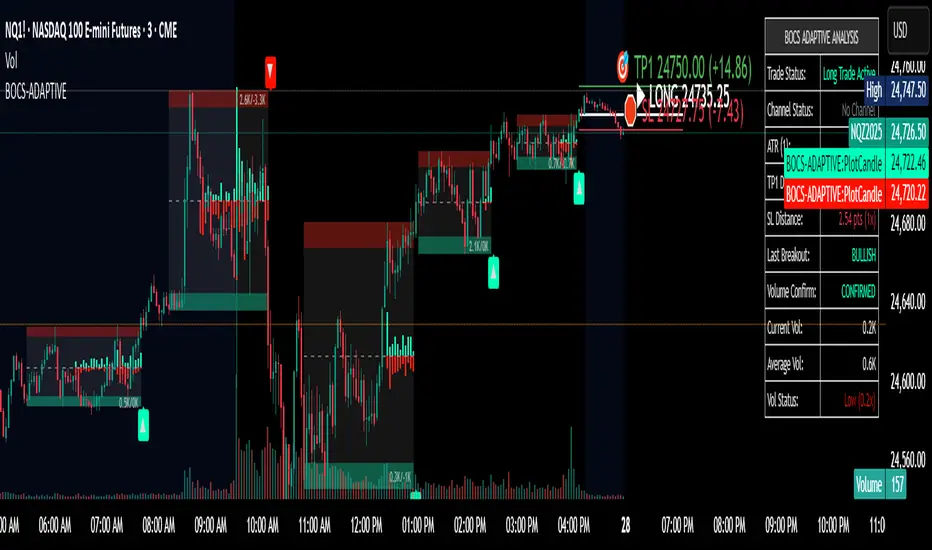
BOCS AdaptiveBOCS Adaptive Strategy - Automated Volatility Breakout System
WHAT THIS STRATEGY DOES:
This is an automated trading strategy that detects consolidation patterns through volatility analysis and executes trades when price breaks out of these channels. Take-profit and stop-loss levels are calculated dynamically using Average True Range (ATR) to adapt to current market volatility. The strategy closes positions partially at the first profit target and exits the remainder at the second target or stop loss.
TECHNICAL METHODOLOGY:
Price Normalization Process:
The strategy begins by normalizing price to create a consistent measurement scale. It calculates the highest high and lowest low over a user-defined lookback period (default 100 bars). The current close price is then normalized using the formula: (close - lowest_low) / (highest_high - lowest_low). This produces values between 0 and 1, allowing volatility analysis to work consistently across different instruments and price levels.
Volatility Detection:
A 14-period standard deviation is applied to the normalized price series. Standard deviation measures how much prices deviate from their average - higher values indicate volatility expansion, lower values indicate consolidation. The strategy uses ta.highestbars() and ta.lowestbars() functions to track when volatility reaches peaks and troughs over the detection length period (default 14 bars).
Channel Formation Logic:
When volatility crosses from a high level to a low level, this signals the beginning of a consolidation phase. The strategy records this moment using ta.crossover(upper, lower) and begins tracking the highest and lowest prices during the consolidation. These become the channel boundaries. The duration between the crossover and current bar must exceed 10 bars minimum to avoid false channels from brief volatility spikes. Channels are drawn using box objects with the recorded high/low boundaries.
Breakout Signal Generation:
Two detection modes are available:
Strong Closes Mode (default): Breakout occurs when the candle body midpoint math.avg(close, open) exceeds the channel boundary. This filters out wick-only breaks.
Any Touch Mode: Breakout occurs when the close price exceeds the boundary.
When price closes above the upper channel boundary, a bullish breakout signal generates. When price closes below the lower boundary, a bearish breakout signal generates. The channel is then removed from the chart.
ATR-Based Risk Management:
The strategy uses request.security() to fetch ATR values from a specified timeframe, which can differ from the chart timeframe. For example, on a 5-minute chart, you can use 1-minute ATR for more responsive calculations. The ATR is calculated using ta.atr(length) with a user-defined period (default 14).
Exit levels are calculated at the moment of breakout:
Long Entry Price = Upper channel boundary
Long TP1 = Entry + (ATR × TP1 Multiplier)
Long TP2 = Entry + (ATR × TP2 Multiplier)
Long SL = Entry - (ATR × SL Multiplier)
For short trades, the calculation inverts:
Short Entry Price = Lower channel boundary
Short TP1 = Entry - (ATR × TP1 Multiplier)
Short TP2 = Entry - (ATR × TP2 Multiplier)
Short SL = Entry + (ATR × SL Multiplier)
Trade Execution Logic:
When a breakout occurs, the strategy checks if trading hours filter is satisfied (if enabled) and if position size equals zero (no existing position). If volume confirmation is enabled, it also verifies that current volume exceeds 1.2 times the 20-period simple moving average.
If all conditions are met:
strategy.entry() opens a position using the user-defined number of contracts
strategy.exit() immediately places a stop loss order
The code monitors price against TP1 and TP2 levels on each bar
When price reaches TP1, strategy.close() closes the specified number of contracts (e.g., if you enter with 3 contracts and set TP1 close to 1, it closes 1 contract). When price reaches TP2, it closes all remaining contracts. If stop loss is hit first, the entire position exits via the strategy.exit() order.
Volume Analysis System:
The strategy uses ta.requestUpAndDownVolume(timeframe) to fetch up volume, down volume, and volume delta from a specified timeframe. Three display modes are available:
Volume Mode: Shows total volume as bars scaled relative to the 20-period average
Comparison Mode: Shows up volume and down volume as separate bars above/below the channel midline
Delta Mode: Shows net volume delta (up volume - down volume) as bars, positive values above midline, negative below
The volume confirmation logic compares breakout bar volume to the 20-period SMA. If volume ÷ average > 1.2, the breakout is classified as "confirmed." When volume confirmation is enabled in settings, only confirmed breakouts generate trades.
INPUT PARAMETERS:
Strategy Settings:
Number of Contracts: Fixed quantity to trade per signal (1-1000)
Require Volume Confirmation: Toggle to only trade signals with volume >120% of average
TP1 Close Contracts: Exact number of contracts to close at first target (1-1000)
Use Trading Hours Filter: Toggle to restrict trading to specified session
Trading Hours: Session input in HHMM-HHMM format (e.g., "0930-1600")
Main Settings:
Normalization Length: Lookback bars for high/low calculation (1-500, default 100)
Box Detection Length: Period for volatility peak/trough detection (1-100, default 14)
Strong Closes Only: Toggle between body midpoint vs close price for breakout detection
Nested Channels: Allow multiple overlapping channels vs single channel at a time
ATR TP/SL Settings:
ATR Timeframe: Source timeframe for ATR calculation (1, 5, 15, 60, etc.)
ATR Length: Smoothing period for ATR (1-100, default 14)
Take Profit 1 Multiplier: Distance from entry as multiple of ATR (0.1-10.0, default 2.0)
Take Profit 2 Multiplier: Distance from entry as multiple of ATR (0.1-10.0, default 3.0)
Stop Loss Multiplier: Distance from entry as multiple of ATR (0.1-10.0, default 1.0)
Enable Take Profit 2: Toggle second profit target on/off
VISUAL INDICATORS:
Channel boxes with semi-transparent fill showing consolidation zones
Green/red colored zones at channel boundaries indicating breakout areas
Volume bars displayed within channels using selected mode
TP/SL lines with labels showing both price level and distance in points
Entry signals marked with up/down triangles at breakout price
Strategy status table showing position, contracts, P&L, ATR values, and volume confirmation status
HOW TO USE:
For 2-Minute Scalping:
Set ATR Timeframe to "1" (1-minute), ATR Length to 12, TP1 Multiplier to 2.0, TP2 Multiplier to 3.0, SL Multiplier to 1.5. Enable volume confirmation and strong closes only. Use trading hours filter to avoid low-volume periods.
For 5-15 Minute Day Trading:
Set ATR Timeframe to match chart or use 5-minute, ATR Length to 14, TP1 Multiplier to 2.0, TP2 Multiplier to 3.5, SL Multiplier to 1.2. Volume confirmation recommended but optional.
For Hourly+ Swing Trading:
Set ATR Timeframe to 15-30 minute, ATR Length to 14-21, TP1 Multiplier to 2.5, TP2 Multiplier to 4.0, SL Multiplier to 1.5. Volume confirmation optional, nested channels can be enabled for multiple setups.
BACKTEST CONSIDERATIONS:
Strategy performs best during trending or volatility expansion phases
Consolidation-heavy or choppy markets produce more false signals
Shorter timeframes require wider stop loss multipliers due to noise
Commission and slippage significantly impact performance on sub-5-minute charts
Volume confirmation generally improves win rate but reduces trade frequency
ATR multipliers should be optimized for specific instrument characteristics
COMPATIBLE MARKETS:
Works on any instrument with price and volume data including forex pairs, stock indices, individual stocks, cryptocurrency, commodities, and futures contracts. Requires TradingView data feed that includes volume for volume confirmation features to function.
KNOWN LIMITATIONS:
Stop losses execute via strategy.exit() and may not fill at exact levels during gaps or extreme volatility
request.security() on lower timeframes requires higher-tier TradingView subscription
False breakouts inherent to breakout strategies cannot be completely eliminated
Performance varies significantly based on market regime (trending vs ranging)
Partial closing logic requires sufficient position size relative to TP1 close contracts setting
RISK DISCLOSURE:
Trading involves substantial risk of loss. Past performance of this or any strategy does not guarantee future results. This strategy is provided for educational purposes and automated backtesting. Thoroughly test on historical data and paper trade before risking real capital. Market conditions change and strategies that worked historically may fail in the future. Use appropriate position sizing and never risk more than you can afford to lose. Consider consulting a licensed financial advisor before making trading decisions.
ACKNOWLEDGMENT & CREDITS:
This strategy is built upon the channel detection methodology created by AlgoAlpha in the "Smart Money Breakout Channels" indicator. Full credit and appreciation to AlgoAlpha for pioneering the normalized volatility approach to identifying consolidation patterns and sharing this innovative technique with the TradingView community. The enhancements added to the original concept include automated trade execution, multi-timeframe ATR-based risk management, partial position closing by contract count, volume confirmation filtering, and real-time position monitoring.
The Best Strategy Template[LuciTech]Hello Traders,
This is a powerful and flexible strategy template designed to help you create, backtest, and deploy your own custom trading strategies. This template is not a ready-to-use strategy but a framework that simplifies the development process by providing a wide range of pre-built features and functionalities.
What It Does
The LuciTech Strategy Template provides a robust foundation for building your own automated trading strategies. It includes a comprehensive set of features that are essential for any serious trading strategy, allowing you to focus on your unique trading logic without having to code everything from scratch.
Key Features
The LuciTech Strategy Template integrates several powerful features to enhance your strategy development:
•
Advanced Risk Management: This includes robust controls for defining your Risk Percentage per Trade, setting a precise Risk-to-Reward Ratio, and implementing an intelligent Breakeven Stop-Loss mechanism that automatically adjusts your stop to the entry price once a specified profit threshold is reached. These elements are crucial for capital preservation and consistent profitability.
•
Flexible Stop-Loss Options: The template offers adaptable stop-loss calculation methods, allowing you to choose between ATR-Based Stop-Loss, which dynamically adjusts to market volatility, and Candle-Based Stop-Loss, which uses structural price points from previous candles. This flexibility ensures the stop-loss strategy aligns with diverse trading styles.
•
Time-Based Filtering: Optimize your strategy's performance by restricting trading activity to specific hours of the day. This feature allows you to avoid unfavorable market conditions or focus on periods of higher liquidity and volatility relevant to your strategy.
•
Customizable Webhook Alerts: Stay informed with advanced notification capabilities. The template supports sending detailed webhook alerts in various JSON formats (Standard, Telegram, Concise Telegram) to external platforms, facilitating real-time monitoring and potential integration with automated trading systems.
•
Comprehensive Visual Customization: Enhance your analytical clarity with extensive visual options. You can customize the colors of entry, stop-loss, and take-profit lines, and effectively visualize market inefficiencies by displaying and customizing Fair Value Gap (FVG) boxes directly on your chart.
How It Does It
The LuciTech Strategy Template is meticulously crafted using Pine Script, TradingView's powerful and expressive programming language. The underlying architecture is designed for clarity and modularity, allowing for straightforward integration of your unique trading signals. At its core, the template operates by taking user-defined entry and exit conditions and then applying a sophisticated layer of risk management, position sizing, and trade execution logic.
For instance, when a longCondition or shortCondition is met, the template dynamically calculates the appropriate position size. This calculation is based on your specified risk_percent of equity and the stop_distance (the distance between your entry price and the calculated stop-loss level). This ensures that each trade adheres to your predefined risk parameters, a critical component of disciplined trading.
The flexibility in stop-loss calculation is achieved through a switch statement that evaluates the sl_type input. Whether you choose an ATR-based stop, which adapts to market volatility, or a candle-based stop, which uses structural price points, the template seamlessly integrates these methods. The ATR calculation itself is further refined by allowing various smoothing methods (RMA, SMA, EMA, WMA), providing granular control over how volatility is measured.
Time-based filtering is implemented by comparing the current bar's time with user-defined start_hour, start_minute, end_hour, and end_minute inputs. This allows the strategy to activate or deactivate trading during specific market sessions or periods of the day, a valuable tool for optimizing performance and avoiding unfavorable conditions.
Furthermore, the template incorporates advanced webhook alert functionality. When a trade is executed, a customizable JSON message is formatted based on your webhook_format selection (Standard, Telegram, or Concise Telegram) and sent via alert function. This enables seamless integration with external services for real-time notifications or even automated trade execution through third-party platforms.
Visual feedback is paramount for understanding strategy behavior. The template utilizes plot and fill functions to clearly display entry prices, stop-loss levels, and take-profit targets directly on the chart. Customizable colors for these elements, along with dedicated options for Fair Value Gap (FVG) boxes, enhance the visual analysis during backtesting and live trading, making it easier to interpret the strategy's actions.
How It's Original
The LuciTech Strategy Template distinguishes itself in the crowded landscape of TradingView scripts through its unique combination of integrated, advanced risk management features, highly flexible stop-loss methodologies, and sophisticated alerting capabilities, all within a user-friendly and modular framework. While many templates offer basic entry/exit signal integration, LuciTech goes several steps further by providing a robust, ready-to-use infrastructure for managing the entire trade lifecycle once a signal is generated.
Unlike templates that might require users to piece together various risk management components or code complex stop-loss logic from scratch, LuciTech offers these critical functionalities out-of-the-box. The inclusion of dynamic position sizing based on a user-defined risk percentage, a configurable risk-to-reward ratio, and an intelligent breakeven mechanism significantly elevates its utility. This comprehensive approach to capital preservation and profit targeting is a cornerstone of professional trading and is often overlooked or simplified in generic templates.
Furthermore, the template's provision for multiple stop-loss calculation types—ATR-based for volatility adaptation, and candle-based for structural support/resistance—demonstrates a deep understanding of diverse trading strategies. The underlying code for these calculations is already implemented, saving developers considerable time and effort. The subtle yet powerful inclusion of FVG (Fair Value Gap) related inputs also hints at advanced price action concepts, offering a sophisticated layer of analysis and execution that is not commonly found in general-purpose templates.
The advanced webhook alerting system, with its support for various JSON formats tailored for platforms like Telegram, showcases an originality in catering to the needs of modern, automated trading setups. This moves beyond simple TradingView pop-up alerts, enabling seamless integration with external systems for real-time trade monitoring and execution. This level of external connectivity and customizable data output is a significant differentiator.
In essence, the LuciTech Strategy Template is original not just in its individual features, but in how these features are cohesively integrated to form a powerful, opinionated, yet highly adaptable system. It empowers traders to focus their creative energy on developing their core entry/exit signals, confident that the underlying framework will handle the complexities of risk management, trade execution, and external communication with precision and flexibility. It's a comprehensive solution designed to accelerate the development of robust and professional trading strategies.
How to Modify the Logic to Apply Your Strategy
The LuciTech Strategy Template is designed with modularity in mind, making it exceptionally straightforward to integrate your unique trading strategy logic. The template provides a clear separation between the core strategy management (risk, position sizing, exits) and the entry signal generation. This allows you to easily plug in your own buy and sell conditions without altering the robust underlying framework.
Here’s a step-by-step guide on how to adapt the template to your specific trading strategy:
1.
Locate the Strategy Logic Section:
Open the Pine Script editor in TradingView and navigate to the section clearly marked with the comment //Strategy Logic Example:. This is where the template’s placeholder entry conditions (a simple moving average crossover) are defined.
2.
Define Your Custom Entry Conditions:
Within this section, you will find variables such as longCondition and shortCondition. These are boolean variables that determine when a long or short trade should be initiated. Replace the existing example logic with your own custom buy and sell conditions. Your conditions can be based on any combination of indicators, price action patterns, candlestick formations, or other market analysis techniques. For example, if your strategy involves a combination of RSI and MACD, you would define longCondition as (rsi > 50 and macd_line > signal_line) and shortCondition as (rsi < 50 and macd_line < signal_line).
3.
Leverage the Template’s Built-in Features:
Once your longCondition and shortCondition are defined, the rest of the template automatically takes over. The integrated risk management module will calculate the appropriate position size based on your Risk % input and the chosen Stop Loss Type. The Risk:Reward ratio will determine your take-profit levels, and the Breakeven at R feature will manage your stop-loss dynamically. The time filter (Use Time Filter) will ensure your trades only occur within your specified hours, and the webhook alerts will notify you of trade executions.

Trendline Breaks with Multi Fibonacci Supertrend StrategyTMFS Strategy: Advanced Trendline Breakouts with Multi-Fibonacci Supertrend
Elevate your algorithmic trading with institutional-grade signal confluence
Strategy Genesis & Evolution
This advanced trading system represents the culmination of a personal research journey, evolving from my custom " Multi Fibonacci Supertrend with Signals " indicator into a comprehensive trading strategy. Built upon the exceptional trendline detection methodology pioneered by LuxAlgo in their " Trendlines with Breaks " indicator, I've engineered a systematic framework that integrates multiple technical factors into a cohesive trading system.
Core Fibonacci Principles
At the heart of this strategy lies the Fibonacci sequence application to volatility measurement:
// Fibonacci-based factors for multiple Supertrend calculations
factor1 = input.float(0.618, 'Factor 1 (Weak/Fibonacci)', minval = 0.01, step = 0.01)
factor2 = input.float(1.618, 'Factor 2 (Medium/Golden Ratio)', minval = 0.01, step = 0.01)
factor3 = input.float(2.618, 'Factor 3 (Strong/Extended Fib)', minval = 0.01, step = 0.01)
These precise Fibonacci ratios create a dynamic volatility envelope that adapts to changing market conditions while maintaining mathematical harmony with natural price movements.
Dynamic Trendline Detection
The strategy incorporates LuxAlgo's pioneering approach to trendline detection:
// Pivotal swing detection (inspired by LuxAlgo)
pivot_high = ta.pivothigh(swing_length, swing_length)
pivot_low = ta.pivotlow(swing_length, swing_length)
// Dynamic slope calculation using ATR
slope = atr_value / swing_length * atr_multiplier
// Update trendlines based on pivot detection
if bool(pivot_high)
upper_slope := slope
upper_trendline := pivot_high
else
upper_trendline := nz(upper_trendline) - nz(upper_slope)
This adaptive trendline approach automatically identifies key structural market boundaries, adjusting in real-time to evolving chart patterns.
Breakout State Management
The strategy implements sophisticated state tracking for breakout detection:
// Track breakouts with state variables
var int upper_breakout_state = 0
var int lower_breakout_state = 0
// Update breakout state when price crosses trendlines
upper_breakout_state := bool(pivot_high) ? 0 : close > upper_trendline ? 1 : upper_breakout_state
lower_breakout_state := bool(pivot_low) ? 0 : close < lower_trendline ? 1 : lower_breakout_state
// Detect new breakouts (state transitions)
bool new_upper_breakout = upper_breakout_state > upper_breakout_state
bool new_lower_breakout = lower_breakout_state > lower_breakout_state
This state-based approach enables precise identification of the exact moment when price breaks through a significant trendline.
Multi-Factor Signal Confluence
Entry signals require confirmation from multiple technical factors:
// Define entry conditions with multi-factor confluence
long_entry_condition = enable_long_positions and
upper_breakout_state > upper_breakout_state and // New trendline breakout
di_plus > di_minus and // Bullish DMI confirmation
close > smoothed_trend // Price above Supertrend envelope
// Execute trades only with full confirmation
if long_entry_condition
strategy.entry('L', strategy.long, comment = "LONG")
This strict requirement for confluence significantly reduces false signals and improves the quality of trade entries.
Advanced Risk Management
The strategy includes sophisticated risk controls with multiple methodologies:
// Calculate stop loss based on selected method
get_long_stop_loss_price(base_price) =>
switch stop_loss_method
'PERC' => base_price * (1 - long_stop_loss_percent)
'ATR' => base_price - long_stop_loss_atr_multiplier * entry_atr
'RR' => base_price - (get_long_take_profit_price() - base_price) / long_risk_reward_ratio
=> na
// Implement trailing functionality
strategy.exit(
id = 'Long Take Profit / Stop Loss',
from_entry = 'L',
qty_percent = take_profit_quantity_percent,
limit = trailing_take_profit_enabled ? na : long_take_profit_price,
stop = long_stop_loss_price,
trail_price = trailing_take_profit_enabled ? long_take_profit_price : na,
trail_offset = trailing_take_profit_enabled ? long_trailing_tp_step_ticks : na,
comment = "TP/SL Triggered"
)
This flexible approach adapts to varying market conditions while providing comprehensive downside protection.
Performance Characteristics
Rigorous backtesting demonstrates exceptional capital appreciation potential with impressive risk-adjusted metrics:
Remarkable total return profile (1,517%+)
Strong Sortino ratio (3.691) indicating superior downside risk control
Profit factor of 1.924 across all trades (2.153 for long positions)
Win rate exceeding 35% with balanced distribution across varied market conditions
Institutional Considerations
The strategy architecture addresses execution complexities faced by institutional participants with temporal filtering and date-range capabilities:
// Time Filter settings with flexible timezone support
import jason5480/time_filters/5 as time_filter
src_timezone = input.string(defval = 'Exchange', title = 'Source Timezone')
dst_timezone = input.string(defval = 'Exchange', title = 'Destination Timezone')
// Date range filtering for precise execution windows
use_from_date = input.bool(defval = true, title = 'Enable Start Date')
from_date = input.time(defval = timestamp('01 Jan 2022 00:00'), title = 'Start Date')
// Validate trading permission based on temporal constraints
date_filter_approved = time_filter.is_in_date_range(
use_from_date, from_date, use_to_date, to_date, src_timezone, dst_timezone
)
These capabilities enable precise execution timing and market session optimization critical for larger market participants.
Acknowledgments
Special thanks to LuxAlgo for the pioneering work on trendline detection and breakout identification that inspired elements of this strategy. Their innovative approach to technical analysis provided a valuable foundation upon which I could build my Fibonacci-based methodology.
This strategy is shared under the same Attribution-NonCommercial-ShareAlike 4.0 International (CC BY-NC-SA 4.0) license as LuxAlgo's original work.
Past performance is not indicative of future results. Conduct thorough analysis before implementing any algorithmic strategy.

Volume Block Order AnalyzerCore Concept
The Volume Block Order Analyzer is a sophisticated Pine Script strategy designed to detect and analyze institutional money flow through large block trades. It identifies unusually high volume candles and evaluates their directional bias to provide clear visual signals of potential market movements.
How It Works: The Mathematical Model
1. Volume Anomaly Detection
The strategy first identifies "block trades" using a statistical approach:
```
avgVolume = ta.sma(volume, lookbackPeriod)
isHighVolume = volume > avgVolume * volumeThreshold
```
This means a candle must have volume exceeding the recent average by a user-defined multiplier (default 2.0x) to be considered a significant block trade.
2. Directional Impact Calculation
For each block trade identified, its price action determines direction:
- Bullish candle (close > open): Positive impact
- Bearish candle (close < open): Negative impact
The magnitude of impact is proportional to the volume size:
```
volumeWeight = volume / avgVolume // How many times larger than average
blockImpact = (isBullish ? 1.0 : -1.0) * (volumeWeight / 10)
```
This creates a normalized impact score typically ranging from -1.0 to 1.0, scaled by dividing by 10 to prevent excessive values.
3. Cumulative Impact with Time Decay
The key innovation is the cumulative impact calculation with decay:
```
cumulativeImpact := cumulativeImpact * impactDecay + blockImpact
```
This mathematical model has important properties:
- Recent block trades have stronger influence than older ones
- Impact gradually "fades" at rate determined by decay factor (default 0.95)
- Sustained directional pressure accumulates over time
- Opposing pressure gradually counteracts previous momentum
Trading Logic
Signal Generation
The strategy generates trading signals based on momentum shifts in institutional order flow:
1. Long Entry Signal: When cumulative impact crosses from negative to positive
```
if ta.crossover(cumulativeImpact, 0)
strategy.entry("Long", strategy.long)
```
*Logic: Institutional buying pressure has overcome selling pressure, indicating potential upward movement*
2. Short Entry Signal: When cumulative impact crosses from positive to negative
```
if ta.crossunder(cumulativeImpact, 0)
strategy.entry("Short", strategy.short)
```
*Logic: Institutional selling pressure has overcome buying pressure, indicating potential downward movement*
3. Exit Logic: Positions are closed when the cumulative impact moves against the position
```
if cumulativeImpact < 0
strategy.close("Long")
```
*Logic: The original signal is no longer valid as institutional flow has reversed*
Visual Interpretation System
The strategy employs multiple visualization techniques:
1. Color Gradient Bar System:
- Deep green: Strong buying pressure (impact > 0.5)
- Light green: Moderate buying pressure (0.1 < impact ≤ 0.5)
- Yellow-green: Mild buying pressure (0 < impact ≤ 0.1)
- Yellow: Neutral (impact = 0)
- Yellow-orange: Mild selling pressure (-0.1 < impact ≤ 0)
- Orange: Moderate selling pressure (-0.5 < impact ≤ -0.1)
- Red: Strong selling pressure (impact ≤ -0.5)
2. Dynamic Impact Line:
- Plots the cumulative impact as a line
- Line color shifts with impact value
- Line movement shows momentum and trend strength
3. Block Trade Labels:
- Marks significant block trades directly on the chart
- Shows direction and volume amount
- Helps identify key moments of institutional activity
4. Information Dashboard:
- Current impact value and signal direction
- Average volume benchmark
- Count of significant block trades
- Min/Max impact range
Benefits and Use Cases
This strategy provides several advantages:
1. Institutional Flow Detection: Identifies where large players are positioning themselves
2. Early Trend Identification: Often detects institutional accumulation/distribution before major price movements
3. Market Context Enhancement: Provides deeper insight than simple price action alone
4. Objective Decision Framework: Quantifies what might otherwise be subjective observations
5. Adaptive to Market Conditions: Works across different timeframes and instruments by using relative volume rather than absolute thresholds
Customization Options
The strategy allows users to fine-tune its behavior:
- Volume Threshold: How unusual a volume spike must be to qualify
- Lookback Period: How far back to measure average volume
- Impact Decay Factor: How quickly older trades lose influence
- Visual Settings: Labels and line width customization
This sophisticated yet intuitive strategy provides traders with a window into institutional activity, helping identify potential trend changes before they become obvious in price action alone.
Friday Bond Short StrategyStrategy: Friday Bond Short Strategy (1H Timeframe)
Objective:
This strategy aims to open short positions on a specified day and hour (Eastern Time) and close those positions on another specified day and hour. The background color of the chart will turn green when a position is active, providing a visual cue of an open trade.
Parameters:
1. Entry Day:
• Defines the day of the week on which the short position will be opened.
• Value: 6 for Friday (Pine Script’s weekday numbering: Monday = 2, Friday = 6).
2. Entry Hour:
• Specifies the hour (Eastern Time) when the short position will be opened.
• Value: 13 for 13:00 ET (1:00 PM).
3. Exit Day:
• Defines the day of the week on which the short position will be closed.
• Value: 2 for Monday.
4. Exit Hour:
• Specifies the hour (Eastern Time) when the position will be closed.
• Value: 13 for 13:00 ET (1:00 PM).
How It Works:
1. Time Adjustment to Eastern Time:
• The script converts all time references to Eastern Time (America/New_York) to ensure the strategy operates according to the desired time zone.
2. Entry Conditions:
• The strategy checks if the current day of the week matches the specified entry_day and if the current hour matches the specified entry_hour.
• If both conditions are met, a short position is opened (strategy.entry("Short", strategy.short)).
3. Exit Conditions:
• Similarly, the strategy checks if the current day of the week matches the specified exit_day and if the current hour matches the specified exit_hour.
• If both conditions are met, the open short position is closed (strategy.close("Short")).
4. Background Color:
• The background color of the chart is adjusted based on whether there is an open position:
• Green Background: If the strategy has an open position (strategy.position_size > 0), the background is set to light green.
• No Background Color: If there is no open position, the background color is not set (na).
Summary:
The Friday Bond Short Strategy is designed to enter short positions on Fridays at 1:00 PM ET and close them on Mondays at 1:00 PM ET. The chart background color turns green when a short position is active, providing a clear visual indication of when the strategy is engaged in a trade.

Supertrend Advance Pullback StrategyHandbook for the Supertrend Advance Strategy
1. Introduction
Purpose of the Handbook:
The main purpose of this handbook is to serve as a comprehensive guide for traders and investors who are looking to explore and harness the potential of the Supertrend Advance Strategy. In the rapidly changing financial market, having the right tools and strategies at one's disposal is crucial. Whether you're a beginner hoping to dive into the world of trading or a seasoned investor aiming to optimize and diversify your portfolio, this handbook offers the insights and methodologies you need. By the end of this guide, readers should have a clear understanding of how the Supertrend Advance Strategy works, its benefits, potential pitfalls, and practical application in various trading scenarios.
Overview of the Supertrend Advance Pullback Strategy:
At its core, the Supertrend Advance Strategy is an evolution of the popular Supertrend Indicator. Designed to generate buy and sell signals in trending markets, the Supertrend Indicator has been a favorite tool for many traders around the world. The Advance Strategy, however, builds upon this foundation by introducing enhanced mechanisms, filters, and methodologies to increase precision and reduce false signals.
1. Basic Concept:
The Supertrend Advance Strategy relies on a combination of price action and volatility to determine the potential trend direction. By assessing the average true range (ATR) in conjunction with specific price points, this strategy aims to highlight the potential starting and ending points of market trends.
2. Methodology:
Unlike the traditional Supertrend Indicator, which primarily focuses on closing prices and ATR, the Advance Strategy integrates other critical market variables, such as volume, momentum oscillators, and perhaps even fundamental data, to validate its signals. This multidimensional approach ensures that the generated signals are more reliable and are less prone to market noise.
3. Benefits:
One of the main benefits of the Supertrend Advance Strategy is its ability to filter out false breakouts and minor price fluctuations, which can often lead to premature exits or entries in the market. By waiting for a confluence of factors to align, traders using this advanced strategy can increase their chances of entering or exiting trades at optimal points.
4. Practical Applications:
The Supertrend Advance Strategy can be applied across various timeframes, from intraday trading to swing trading and even long-term investment scenarios. Furthermore, its flexible nature allows it to be tailored to different asset classes, be it stocks, commodities, forex, or cryptocurrencies.
In the subsequent sections of this handbook, we will delve deeper into the intricacies of this strategy, offering step-by-step guidelines on its application, case studies, and tips for maximizing its efficacy in the volatile world of trading.
As you journey through this handbook, we encourage you to approach the Supertrend Advance Strategy with an open mind, testing and tweaking it as per your personal trading style and risk appetite. The ultimate goal is not just to provide you with a new tool but to empower you with a holistic strategy that can enhance your trading endeavors.
2. Getting Started
Navigating the financial markets can be a daunting task without the right tools. This section is dedicated to helping you set up the Supertrend Advance Strategy on one of the most popular charting platforms, TradingView. By following the steps below, you'll be able to integrate this strategy into your charts and start leveraging its insights in no time.
Setting up on TradingView:
TradingView is a web-based platform that offers a wide range of charting tools, social networking, and market data. Before you can apply the Supertrend Advance Strategy, you'll first need a TradingView account. If you haven't set one up yet, here's how:
1. Account Creation:
• Visit TradingView's official website.
• Click on the "Join for free" or "Sign up" button.
• Follow the registration process, providing the necessary details and setting up your login credentials.
2. Navigating the Dashboard:
• Once logged in, you'll be taken to your dashboard. Here, you'll see a variety of tools, including watchlists, alerts, and the main charting window.
• To begin charting, type in the name or ticker of the asset you're interested in the search bar at the top.
3. Configuring Chart Settings:
• Before integrating the Supertrend Advance Strategy, familiarize yourself with the chart settings. This can be accessed by clicking the 'gear' icon on the top right of the chart window.
• Adjust the chart type, time intervals, and other display settings to your preference.
Integrating the Strategy into a Chart:
Now that you're set up on TradingView, it's time to integrate the Supertrend Advance Strategy.
1. Accessing the Pine Script Editor:
• Located at the top-center of your screen, you'll find the "Pine Editor" tab. Click on it.
• This is where custom strategies and indicators are scripted or imported.
2. Loading the Supertrend Advance Strategy Script:
• Depending on whether you have the script or need to find it, there are two paths:
• If you have the script: Copy the Supertrend Advance Strategy script, and then paste it into the Pine Editor.
• If searching for the script: Click on the “Indicators” icon (looks like a flame) at the top of your screen, and then type “Supertrend Advance Strategy” in the search bar. If available, it will show up in the list. Simply click to add it to your chart.
3. Applying the Strategy:
• After pasting or selecting the Supertrend Advance Strategy in the Pine Editor, click on the “Add to Chart” button located at the top of the editor. This will overlay the strategy onto your main chart window.
4. Configuring Strategy Settings:
• Once the strategy is on your chart, you'll notice a small settings ('gear') icon next to its name in the top-left of the chart window. Click on this to access settings.
• Here, you can adjust various parameters of the Supertrend Advance Strategy to better fit your trading style or the specific asset you're analyzing.
5. Interpreting Signals:
• With the strategy applied, you'll now see buy/sell signals represented on your chart. Take time to familiarize yourself with how these look and behave over various timeframes and market conditions.
3. Strategy Overview
What is the Supertrend Advance Strategy?
The Supertrend Advance Strategy is a refined version of the classic Supertrend Indicator, which was developed to aid traders in spotting market trends. The strategy utilizes a combination of data points, including average true range (ATR) and price momentum, to generate buy and sell signals.
In essence, the Supertrend Advance Strategy can be visualized as a line that moves with the price. When the price is above the Supertrend line, it indicates an uptrend and suggests a potential buy position. Conversely, when the price is below the Supertrend line, it hints at a downtrend, suggesting a potential selling point.
Strategy Goals and Objectives:
1. Trend Identification: At the core of the Supertrend Advance Strategy is the goal to efficiently and consistently identify prevailing market trends. By recognizing these trends, traders can position themselves to capitalize on price movements in their favor.
2. Reducing Noise: Financial markets are often inundated with 'noise' - short-term price fluctuations that can mislead traders. The Supertrend Advance Strategy aims to filter out this noise, allowing for clearer decision-making.
3. Enhancing Risk Management: With clear buy and sell signals, traders can set more precise stop-loss and take-profit points. This leads to better risk management and potentially improved profitability.
4. Versatility: While primarily used for trend identification, the strategy can be integrated with other technical tools and indicators to create a comprehensive trading system.
Type of Assets/Markets to Apply the Strategy:
1. Equities: The Supertrend Advance Strategy is highly popular among stock traders. Its ability to capture long-term trends makes it particularly useful for those trading individual stocks or equity indices.
2. Forex: Given the 24-hour nature of the Forex market and its propensity for trends, the Supertrend Advance Strategy is a valuable tool for currency traders.
3. Commodities: Whether it's gold, oil, or agricultural products, commodities often move in extended trends. The strategy can help in identifying and capitalizing on these movements.
4. Cryptocurrencies: The volatile nature of cryptocurrencies means they can have pronounced trends. The Supertrend Advance Strategy can aid crypto traders in navigating these often tumultuous waters.
5. Futures & Options: Traders and investors in derivative markets can utilize the strategy to make more informed decisions about contract entries and exits.
It's important to note that while the Supertrend Advance Strategy can be applied across various assets and markets, its effectiveness might vary based on market conditions, timeframe, and the specific characteristics of the asset in question. As always, it's recommended to use the strategy in conjunction with other analytical tools and to backtest its effectiveness in specific scenarios before committing to trades.
4. Input Settings
Understanding and correctly configuring input settings is crucial for optimizing the Supertrend Advance Strategy for any specific market or asset. These settings, when tweaked correctly, can drastically impact the strategy's performance.
Grouping Inputs:
Before diving into individual input settings, it's important to group similar inputs. Grouping can simplify the user interface, making it easier to adjust settings related to a specific function or indicator.
Strategy Choice:
This input allows traders to select from various strategies that incorporate the Supertrend indicator. Options might include "Supertrend with RSI," "Supertrend with MACD," etc. By choosing a strategy, the associated input settings for that strategy become available.
Supertrend Settings:
1. Multiplier: Typically, a default value of 3 is used. This multiplier is used in the ATR calculation. Increasing it makes the Supertrend line further from prices, while decreasing it brings the line closer.
2. Period: The number of bars used in the ATR calculation. A common default is 7.
EMA Settings (Exponential Moving Average):
1. Period: Defines the number of previous bars used to calculate the EMA. Common periods are 9, 21, 50, and 200.
2. Source: Allows traders to choose which price (Open, Close, High, Low) to use in the EMA calculation.
RSI Settings (Relative Strength Index):
1. Length: Determines how many periods are used for RSI calculation. The standard setting is 14.
2. Overbought Level: The threshold at which the asset is considered overbought, typically set at 70.
3. Oversold Level: The threshold at which the asset is considered oversold, often at 30.
MACD Settings (Moving Average Convergence Divergence):
1. Short Period: The shorter EMA, usually set to 12.
2. Long Period: The longer EMA, commonly set to 26.
3. Signal Period: Defines the EMA of the MACD line, typically set at 9.
CCI Settings (Commodity Channel Index):
1. Period: The number of bars used in the CCI calculation, often set to 20.
2. Overbought Level: Typically set at +100, denoting overbought conditions.
3. Oversold Level: Usually set at -100, indicating oversold conditions.
SL/TP Settings (Stop Loss/Take Profit):
1. SL Multiplier: Defines the multiplier for the average true range (ATR) to set the stop loss.
2. TP Multiplier: Defines the multiplier for the average true range (ATR) to set the take profit.
Filtering Conditions:
This section allows traders to set conditions to filter out certain signals. For example, one might only want to take buy signals when the RSI is below 30, ensuring they buy during oversold conditions.
Trade Direction and Backtest Period:
1. Trade Direction: Allows traders to specify whether they want to take long trades, short trades, or both.
2. Backtest Period: Specifies the time range for backtesting the strategy. Traders can choose from options like 'Last 6 months,' 'Last 1 year,' etc.
It's essential to remember that while default settings are provided for many of these tools, optimal settings can vary based on the market, timeframe, and trading style. Always backtest new settings on historical data to gauge their potential efficacy.
5. Understanding Strategy Conditions
Developing an understanding of the conditions set within a trading strategy is essential for traders to maximize its potential. Here, we delve deep into the logic behind these conditions, using the Supertrend Advance Strategy as our focal point.
Basic Logic Behind Conditions:
Every strategy is built around a set of conditions that provide buy or sell signals. The conditions are based on mathematical or statistical methods and are rooted in the study of historical price data. The fundamental idea is to recognize patterns or behaviors that have been profitable in the past and might be profitable in the future.
Buy and Sell Conditions:
1. Buy Conditions: Usually formulated around bullish signals or indicators suggesting upward price momentum.
2. Sell Conditions: Centered on bearish signals or indicators indicating downward price momentum.
Simple Strategy:
The simple strategy could involve using just the Supertrend indicator. Here:
• Buy: When price closes above the Supertrend line.
• Sell: When price closes below the Supertrend line.
Pullback Strategy:
This strategy capitalizes on price retracements:
• Buy: When the price retraces to the Supertrend line after a bullish signal and is supported by another bullish indicator.
• Sell: When the price retraces to the Supertrend line after a bearish signal and is confirmed by another bearish indicator.
Indicators Used:
EMA (Exponential Moving Average):
• Logic: EMA gives more weight to recent prices, making it more responsive to current price movements. A shorter-period EMA crossing above a longer-period EMA can be a bullish sign, while the opposite is bearish.
RSI (Relative Strength Index):
• Logic: RSI measures the magnitude of recent price changes to analyze overbought or oversold conditions. Values above 70 are typically considered overbought, and values below 30 are considered oversold.
MACD (Moving Average Convergence Divergence):
• Logic: MACD assesses the relationship between two EMAs of a security’s price. The MACD line crossing above the signal line can be a bullish signal, while crossing below can be bearish.
CCI (Commodity Channel Index):
• Logic: CCI compares a security's average price change with its average price variation. A CCI value above +100 may mean the price is overbought, while below -100 might signify an oversold condition.
And others...
As the strategy expands or contracts, more indicators might be added or removed. The crucial point is to understand the core logic behind each, ensuring they align with the strategy's objectives.
Logic Behind Each Indicator:
1. EMA: Emphasizes recent price movements; provides dynamic support and resistance levels.
2. RSI: Indicates overbought and oversold conditions based on recent price changes.
3. MACD: Showcases momentum and direction of a trend by comparing two EMAs.
4. CCI: Measures the difference between a security's price change and its average price change.
Understanding strategy conditions is not just about knowing when to buy or sell but also about comprehending the underlying market dynamics that those conditions represent. As you familiarize yourself with each condition and indicator, you'll be better prepared to adapt and evolve with the ever-changing financial markets.
6. Trade Execution and Management
Trade execution and management are crucial aspects of any trading strategy. Efficient execution can significantly impact profitability, while effective management can preserve capital during adverse market conditions. In this section, we'll explore the nuances of position entry, exit strategies, and various Stop Loss (SL) and Take Profit (TP) methodologies within the Supertrend Advance Strategy.
Position Entry:
Effective trade entry revolves around:
1. Timing: Enter at a point where the risk-reward ratio is favorable. This often corresponds to confirmatory signals from multiple indicators.
2. Volume Analysis: Ensure there's adequate volume to support the movement. Volume can validate the strength of a signal.
3. Confirmation: Use multiple indicators or chart patterns to confirm the entry point. For instance, a buy signal from the Supertrend indicator can be confirmed with a bullish MACD crossover.
Position Exit Strategies:
A successful exit strategy will lock in profits and minimize losses. Here are some strategies:
1. Fixed Time Exit: Exiting after a predetermined period.
2. Percentage-based Profit Target: Exiting after a certain percentage gain.
3. Indicator-based Exit: Exiting when an indicator gives an opposing signal.
Percentage-based SL/TP:
• Stop Loss (SL): Set a fixed percentage below the entry price to limit potential losses.
• Example: A 2% SL on an entry at $100 would trigger a sell at $98.
• Take Profit (TP): Set a fixed percentage above the entry price to lock in gains.
• Example: A 5% TP on an entry at $100 would trigger a sell at $105.
Supertrend-based SL/TP:
• Stop Loss (SL): Position the SL at the Supertrend line. If the price breaches this line, it could indicate a trend reversal.
• Take Profit (TP): One could set the TP at a point where the Supertrend line flattens or turns, indicating a possible slowdown in momentum.
Swing high/low-based SL/TP:
• Stop Loss (SL): For a long position, set the SL just below the recent swing low. For a short position, set it just above the recent swing high.
• Take Profit (TP): For a long position, set the TP near a recent swing high or resistance. For a short position, near a swing low or support.
And other methods...
1. Trailing Stop Loss: This dynamic SL adjusts with the price movement, locking in profits as the trade moves in your favor.
2. Multiple Take Profits: Divide the position into segments and set multiple TP levels, securing profits in stages.
3. Opposite Signal Exit: Exit when another reliable indicator gives an opposite signal.
Trade execution and management are as much an art as they are a science. They require a blend of analytical skill, discipline, and intuition. Regularly reviewing and refining your strategies, especially in light of changing market conditions, is crucial to maintaining consistent trading performance.
7. Visual Representations
Visual tools are essential for traders, as they simplify complex data into an easily interpretable format. Properly analyzing and understanding the plots on a chart can provide actionable insights and a more intuitive grasp of market conditions. In this section, we’ll delve into various visual representations used in the Supertrend Advance Strategy and their significance.
Understanding Plots on the Chart:
Charts are the primary visual aids for traders. The arrangement of data points, lines, and colors on them tell a story about the market's past, present, and potential future moves.
1. Data Points: These represent individual price actions over a specific timeframe. For instance, a daily chart will have data points showing the opening, closing, high, and low prices for each day.
2. Colors: Used to indicate the nature of price movement. Commonly, green is used for bullish (upward) moves and red for bearish (downward) moves.
Trend Lines:
Trend lines are straight lines drawn on a chart that connect a series of price points. Their significance:
1. Uptrend Line: Drawn along the lows, representing support. A break below might indicate a trend reversal.
2. Downtrend Line: Drawn along the highs, indicating resistance. A break above might suggest the start of a bullish trend.
Filled Areas:
These represent a range between two values on a chart, usually shaded or colored. For instance:
1. Bollinger Bands: The area between the upper and lower band is filled, giving a visual representation of volatility.
2. Volume Profile: Can show a filled area representing the amount of trading activity at different price levels.
Stop Loss and Take Profit Lines:
These are horizontal lines representing pre-determined exit points for trades.
1. Stop Loss Line: Indicates the level at which a trade will be automatically closed to limit losses. Positioned according to the trader's risk tolerance.
2. Take Profit Line: Denotes the target level to lock in profits. Set according to potential resistance (for long trades) or support (for short trades) or other technical factors.
Trailing Stop Lines:
A trailing stop is a dynamic form of stop loss that moves with the price. On a chart:
1. For Long Trades: Starts below the entry price and moves up with the price but remains static if the price falls, ensuring profits are locked in.
2. For Short Trades: Starts above the entry price and moves down with the price but remains static if the price rises.
Visual representations offer traders a clear, organized view of market dynamics. Familiarity with these tools ensures that traders can quickly and accurately interpret chart data, leading to more informed decision-making. Always ensure that the visual aids used resonate with your trading style and strategy for the best results.
8. Backtesting
Backtesting is a fundamental process in strategy development, enabling traders to evaluate the efficacy of their strategy using historical data. It provides a snapshot of how the strategy would have performed in past market conditions, offering insights into its potential strengths and vulnerabilities. In this section, we'll explore the intricacies of setting up and analyzing backtest results and the caveats one must be aware of.
Setting Up Backtest Period:
1. Duration: Determine the timeframe for the backtest. It should be long enough to capture various market conditions (bullish, bearish, sideways). For instance, if you're testing a daily strategy, consider a period of several years.
2. Data Quality: Ensure the data source is reliable, offering high-resolution and clean data. This is vital to get accurate backtest results.
3. Segmentation: Instead of a continuous period, sometimes it's helpful to backtest over distinct market phases, like a particular bear or bull market, to see how the strategy holds up in different environments.
Analyzing Backtest Results:
1. Performance Metrics: Examine metrics like the total return, annualized return, maximum drawdown, Sharpe ratio, and others to gauge the strategy's efficiency.
2. Win Rate: It's the ratio of winning trades to total trades. A high win rate doesn't always signify a good strategy; it should be evaluated in conjunction with other metrics.
3. Risk/Reward: Understand the average profit versus the average loss per trade. A strategy might have a low win rate but still be profitable if the average gain far exceeds the average loss.
4. Drawdown Analysis: Review the periods of losses the strategy could incur and how long it takes, on average, to recover.
9. Tips and Best Practices
Successful trading requires more than just knowing how a strategy works. It necessitates an understanding of when to apply it, how to adjust it to varying market conditions, and the wisdom to recognize and avoid common pitfalls. This section offers insightful tips and best practices to enhance the application of the Supertrend Advance Strategy.
When to Use the Strategy:
1. Market Conditions: Ideally, employ the Supertrend Advance Strategy during trending market conditions. This strategy thrives when there are clear upward or downward trends. It might be less effective during consolidative or sideways markets.
2. News Events: Be cautious around significant news events, as they can cause extreme volatility. It might be wise to avoid trading immediately before and after high-impact news.
3. Liquidity: Ensure you are trading in assets/markets with sufficient liquidity. High liquidity ensures that the price movements are more reflective of genuine market sentiment and not due to thin volume.
Adjusting Settings for Different Markets/Timeframes:
1. Markets: Each market (stocks, forex, commodities) has its own characteristics. It's essential to adjust the strategy's parameters to align with the market's volatility and liquidity.
2. Timeframes: Shorter timeframes (like 1-minute or 5-minute charts) tend to have more noise. You might need to adjust the settings to filter out false signals. Conversely, for longer timeframes (like daily or weekly charts), you might need to be more responsive to genuine trend changes.
3. Customization: Regularly review and tweak the strategy's settings. Periodic adjustments can ensure the strategy remains optimized for the current market conditions.
10. Frequently Asked Questions (FAQs)
Given the complexities and nuances of the Supertrend Advance Strategy, it's only natural for traders, both new and seasoned, to have questions. This section addresses some of the most commonly asked questions regarding the strategy.
1. What exactly is the Supertrend Advance Strategy?
The Supertrend Advance Strategy is an evolved version of the traditional Supertrend indicator. It's designed to provide clearer buy and sell signals by incorporating additional indicators like EMA, RSI, MACD, CCI, etc. The strategy aims to capitalize on market trends while minimizing false signals.
2. Can I use the Supertrend Advance Strategy for all asset types?
Yes, the strategy can be applied to various asset types like stocks, forex, commodities, and cryptocurrencies. However, it's crucial to adjust the settings accordingly to suit the specific characteristics and volatility of each asset type.
3. Is this strategy suitable for day trading?
Absolutely! The Supertrend Advance Strategy can be adjusted to suit various timeframes, making it versatile for both day trading and long-term trading. Remember to fine-tune the settings to align with the timeframe you're trading on.
4. How do I deal with false signals?
No strategy is immune to false signals. However, by combining the Supertrend with other indicators and adhering to strict risk management protocols, you can minimize the impact of false signals. Always use stop-loss orders and consider filtering trades with additional confirmation signals.
5. Do I need any prior trading experience to use this strategy?
While the Supertrend Advance Strategy is designed to be user-friendly, having a foundational understanding of trading and market analysis can greatly enhance your ability to employ the strategy effectively. If you're a beginner, consider pairing the strategy with further education and practice on demo accounts.
6. How often should I review and adjust the strategy settings?
There's no one-size-fits-all answer. Some traders adjust settings weekly, while others might do it monthly. The key is to remain responsive to changing market conditions. Regular backtesting can give insights into potential required adjustments.
7. Can the Supertrend Advance Strategy be automated?
Yes, many traders use algorithmic trading platforms to automate their strategies, including the Supertrend Advance Strategy. However, always monitor automated systems regularly to ensure they're operating as intended.
8. Are there any markets or conditions where the strategy shouldn't be used?
The strategy might generate more false signals in markets that are consolidative or range-bound. During significant news events or times of unexpected high volatility, it's advisable to tread with caution or stay out of the market.
9. How important is backtesting with this strategy?
Backtesting is crucial as it allows traders to understand how the strategy would have performed in the past, offering insights into potential profitability and areas of improvement. Always backtest any new setting or tweak before applying it to live trades.
10. What if the strategy isn't working for me?
No strategy guarantees consistent profits. If it's not working for you, consider reviewing your settings, seeking expert advice, or complementing the Supertrend Advance Strategy with other analysis methods. Remember, continuous learning and adaptation are the keys to trading success.
Other comments
Value of combining several indicators in this script and how they work together
Diversification of Signals: Just as diversifying an investment portfolio can reduce risk, using multiple indicators can offer varied perspectives on potential price movements. Each indicator can capture a different facet of the market, ensuring that traders are not overly reliant on a single data point.
Confirmation & Reduced False Signals: A common challenge with many indicators is the potential for false signals. By requiring confirmation from multiple indicators before acting, the chances of acting on a false signal can be significantly reduced.
Flexibility Across Market Conditions: Different indicators might perform better under different market conditions. For example, while moving averages might excel in trending markets, oscillators like RSI might be more useful during sideways or range-bound conditions. A mashup strategy can potentially adapt better to varying market scenarios.
Comprehensive Analysis: With multiple indicators, traders can gauge trend strength, momentum, volatility, and potential market reversals all at once, providing a holistic view of the market.
How do the different indicators in the Supertrend Advance Strategy work together?
Supertrend: This is primarily a trend-following indicator. It provides traders with buy and sell signals based on the volatility of the price. When combined with other indicators, it can filter out noise and give more weight to strong, confirmed trends.
EMA (Exponential Moving Average): EMA gives more weight to recent price data. It can be used to identify the direction and strength of a trend. When the price is above the EMA, it's generally considered bullish, and vice versa.
RSI (Relative Strength Index): An oscillator that measures the magnitude of recent price changes to evaluate overbought or oversold conditions. By cross-referencing with other indicators like EMA or MACD, traders can spot potential reversals or confirmations of a trend.
MACD (Moving Average Convergence Divergence): This indicator identifies changes in the strength, direction, momentum, and duration of a trend in a stock's price. When the MACD line crosses above the signal line, it can be a bullish sign, and when it crosses below, it can be bearish. Pairing MACD with Supertrend can provide dual confirmation of a trend.
CCI (Commodity Channel Index): Initially developed for commodities, CCI can indicate overbought or oversold conditions. It can be used in conjunction with other indicators to determine entry and exit points.
In essence, the synergy of these indicators provides a balanced, comprehensive approach to trading. Each indicator offers its unique lens into market conditions, and when they align, it can be a powerful indication of a trading opportunity. This combination not only reduces the potential drawbacks of each individual indicator but leverages their strengths, aiming for more consistent and informed trading decisions.
Backtesting and Default Settings
• This indicator has been optimized to be applied for 1 hour-charts. However, the underlying principles of this strategy are supply and demand in the financial markets and the strategy can be applied to all timeframes. Daytraders can use the 1min- or 5min charts, swing-traders can use the daily charts.
• This strategy has been designed to identify the most promising, highest probability entries and trades for each stock or other financial security.
• The combination of the qualifiers results in a highly selective strategy which only considers the most promising swing-trading entries. As a result, you will normally only find a low number of trades for each stock or other financial security per year in case you apply this strategy for the daily charts. Shorter timeframes will result in a higher number of trades / year.
• Consequently, traders need to apply this strategy for a full watchlist rather than just one financial security.
• Default properties: RSI on (length 14, RSI buy level 50, sell level 50), EMA, RSI, MACD on, type of strategy pullback, SL/TP type: ATR (length 10, factor 3), trade direction both, quantity 5, take profit swing hl 5.1, highest / lowest lookback 2, enable ATR trail (ATR length 10, SL ATR multiplier 1.4, TP multiplier 2.1, lookback = 4, trade direction = both).
[MT] Strategy Backtest Template| Initial Release | | EN |
An update of my old script, this script is designed so that it can be used as a template for all those traders who want to save time when programming their strategy and backtesting it, having functions already programmed that in normal development would take you more time to program, with this template you can simply add your favorite indicator and thus be able to take advantage of all the functions that this template has.
🔴Stop Loss and 🟢Take Profit:
No need to mention that it is a Stop Loss and a Take Profit, within these functions we find the options of: fixed percentage (%), fixed price ($), ATR, especially for Stop Loss we find the Pivot Points, in addition to this, the price range between the entry and the Stop Loss can be converted into a trailing stop loss, instead, especially for the Take Profit we have an option to choose a 1:X ratio that complements very well with the Pivot Points.
📈Heikin Ashi Based Entries:
Heikin Ashi entries are trades that are calculated based on Heikin Ashi candles but their price is executed to Japanese candles, thus avoiding false results that occur in Heikin candlestick charts, this making in certain cases better results in strategies that are executed with this option compared to Japanese candlesticks.
📊Dashboard:
A more visual and organized way to see the results and necessary data produced by our strategy, among them we can see the dates between which our operations are made regardless if you have activated some time filter, usual data such as Profit, Win Rate, Profit factor are also displayed in this panel, additionally data such as the total number of operations, how many were gains and how many losses, the average profit and loss for each operation and finally the maximum profits and losses followed, which are data that will be very useful to us when we elaborate our strategies.
Feel free to use this template to program your own strategies, if you find errors or want to request a new feature let me know in the comments or through my social networks found in my tradingview profile.
| Update 1.1 | | EN |
➕Additions: '
Time sessions filter and days of the week filter added to the time filter section.
Option to add leverage to the strategy.
5 Moving Averages, RSI, Stochastic RSI, ADX, and Parabolic Sar have been added as indicators for the strategy.
You can choose from the 6 available indicators the way to trade, entry alert or entry filter.
Added the option of ATR for Take Profit.
Ticker information and timeframe are now displayed on the dashboard.
Added display customization and color customization of indicator plots.
Added customization of display and color plots of trades displayed on chart.
📝Changes:
Now when activating the time filter it is optional to add a start or end date and time, being able to only add a start date or only an end date.
Operation plots have been changed from plot() to line creation with line.new().
Indicator plots can now be controlled from the "plots" section.
Acceptable and deniable range of profit, winrate and profit factor can now be chosen from the "plots" section to be displayed on the dashboard.
Aesthetic changes in the section separations within the settings section and within the code itself.
The function that made the indicators give inputs based on heikin ashi candles has been changed, see the code for more information.
⚙️Fixes:
Dashboard label now projects correctly on all timeframes including custom timeframes.
Removed unnecessary lines and variables to take up less code space.
All code in general has been optimized to avoid the use of variables, unnecessary lines and avoid unnecessary calculations, freeing up space to declare more variables and be able to use fewer lines of code.
| Lanzamiento Inicial | | ES |
Una actualización de mi antiguo script, este script está diseñado para que pueda ser usado como una plantilla para todos aquellos traders que quieran ahorrar tiempo al programar su estrategia y hacer un backtesting de ella, teniendo funciones ya programadas que en el desarrollo normal te tomaría más tiempo programar, con esta plantilla puedes simplemente agregar tu indicador favorito y así poder aprovechar todas las funciones que tiene esta plantilla.
🔴Stop Loss y 🟢Take Profit:
No hace falta mencionar que es un Stop Loss y un Take Profit, dentro de estas funciones encontramos las opciones de: porcentaje fijo (%), precio fijo ($), ATR, en especial para Stop Loss encontramos los Pivot Points, adicionalmente a esto, el rango de precio entre la entrada y el Stop Loss se puede convertir en un trailing stop loss, en cambio, especialmente para el Take Profit tenemos una opción para elegir un ratio 1:X que se complementa muy bien con los Pivot Points.
📈Entradas Basadas en Heikin Ashi:
Las entradas Heikin Ashi son operaciones que son calculados en base a las velas Heikin Ashi pero su precio esta ejecutado a velas japonesas, evitando así́ los falsos resultados que se producen en graficas de velas Heikin, esto haciendo que en ciertos casos se obtengan mejores resultados en las estrategias que son ejecutadas con esta opción en comparación con las velas japonesas.
📊Panel de Control:
Una manera más visual y organizada de ver los resultados y datos necesarios producidos por nuestra estrategia, entre ellos podemos ver las fechas entre las que se hacen nuestras operaciones independientemente si se tiene activado algún filtro de tiempo, datos usuales como el Profit, Win Rate, Profit factor también son mostrados en este panel, adicionalmente se agregaron datos como el número total de operaciones, cuantos fueron ganancias y cuantos perdidas, el promedio de ganancias y pérdidas por cada operación y por ultimo las máximas ganancias y pérdidas seguidas, que son datos que nos serán muy útiles al elaborar nuestras estrategias.
Siéntete libre de usar esta plantilla para programar tus propias estrategias, si encuentras errores o quieres solicitar una nueva función házmelo saber en los comentarios o a través de mis redes sociales que se encuentran en mi perfil de tradingview.
| Actualización 1.1 | | ES |
➕Añadidos:
Filtro de sesiones de tiempo y filtro de días de la semana agregados al apartado de filtro de tiempo.
Opción para agregar apalancamiento a la estrategia.
5 Moving Averages, RSI, Stochastic RSI, ADX, y Parabolic Sar se han agregado como indicadores para la estrategia.
Puedes escoger entre los 6 indicadores disponibles la forma de operar, alerta de entrada o filtro de entrada.
Añadido la opción de ATR para Take Profit.
La información del ticker y la temporalidad ahora se muestran en el dashboard.
Añadido personalización de visualización y color de los plots de indicadores.
Añadido personalización de visualización y color de los plots de operaciones mostradas en grafica.
📝Cambios:
Ahora al activar el filtro de tiempo es opcional añadir una fecha y hora de inicio o fin, pudiendo únicamente agregar una fecha de inicio o solamente una fecha de fin.
Los plots de operaciones han cambiados de plot() a creación de líneas con line.new().
Los plots de indicadores ahora se pueden controlar desde el apartado "plots".
Ahora se puede elegir el rango aceptable y negable de profit, winrate y profit factor desde el apartado "plots" para mostrarse en el dashboard.
Cambios estéticos en las separaciones de secciones dentro del apartado de configuraciones y dentro del propio código.
Se ha cambiado la función que hacía que los indicadores dieran entradas en base a velas heikin ashi, mire el código para más información.
⚙️Arreglos:
El dashboard label ahora se proyecta correctamente en todas las temporalidades incluyendo las temporalidades personalizadas.
Se han eliminado líneas y variables innecesarias para ocupar menos espacio en el código.
Se ha optimizado todo el código en general para evitar el uso de variables, líneas innecesarias y evitar los cálculos innecesarios, liberando espacio para declarar más variables y poder utilizar menos líneas de código.

Portfolio Backtester Engine█ OVERVIEW
Portfolio Backtester Engine (PBTE). This tool will allow you to backtest strategies across multiple securities at once. Allowing you to easier understand if your strategy is robust. If you are familiar with the PineCoders backtesting engine , then you will find this indicator pleasant to work with as it is an adaptation based on that work. Much of the functionality has been kept the same, or enhanced, with some minor adjustments I made on the account of creating a more subjectively intuitive tool.
█ HISTORY
The original purpose of the backtesting engine (`BTE`) was to bridge the gap between strategies and studies . Previously, strategies did not contain the ability to send alerts, but were necessary for backtesting. Studies on the other hand were necessary for sending alerts, but could not provide backtesting results . Often, traders would have to manage two separate Pine scripts to take advantage of each feature, this was less than ideal.
The `BTE` published by PineCoders offered a solution to this issue by generating backtesting results under the context of a study(). This allowed traders to backtest their strategy and simultaneously generate alerts for automated trading, thus eliminating the need for a separate strategy() script (though, even converting the engine to a strategy was made simple by the PineCoders!).
Fast forward a couple years and PineScript evolved beyond these issues and alerts were introduced into strategies. The BTE was not quite as necessary anymore, but is still extremely useful as it contains extra features and data not found under the strategy() context. Below is an excerpt of features contained by the BTE:
"""
More than `40` built-in strategies,
Customizable components,
Coupling with your own external indicator,
Simple conversion from Study to Strategy modes,
Post-Exit analysis to search for alternate trade outcomes,
Use of the Data Window to show detailed bar by bar trade information and global statistics, including some not provided by TV backtesting,
Plotting of reminders and generation of alerts on in-trade events.
"""
Before I go any further, I want to be clear that the BTE is STILL a good tool and it is STILL very useful. The Portfolio Backtesting Engine I am introducing is only a tangental advancement and not to be confused as a replacement, this tool would not have been possible without the `BTE`.
█ THE PROBLEM
Most strategies built in Pine are limited by one thing. Data. Backtesting should be a rigorous process and researchers should examine the performance of their strategy across all market regimes; that includes, bullish and bearish markets, ranging markets, low volatility and high volatility. Depending on your TV subscription The Pine Engine is limited to 5k-20k historical bars available for backtesting, which can often leave the strategy results wanting. As a general rule of thumb, strategies should be tested across a quantity of historical bars which will allow for at least 100 trades. In many cases, the lack of historical bars available for backtesting and frequency of the strategy signals produces less than 100 trades, rendering your strategy results inconclusive.
█ THE SOLUTION
In order to be confident that we have a robust strategy we must test it across all market regimes and we must have over 100 trades. To do this effectively, researchers can use the Portfolio Backtesting Engine (PBTE).
By testing a strategy across a carefully selected portfolio of securities, researchers can now gather 5k-20k historical bars per security! Currently, the PTBE allows up to 5 securities, which amounts to 25k-100k historical bars.
█ HOW TO USE
1 — Add the indicator to your chart.
• Confirm inputs. These will be the most important initial values which you can change later by clicking the gear icon ⚙ and opening up the settings of the indicator.
2 — Select a portfolio.
• You will want to spend some time carefully selecting a portfolio of securities.
• Each security should be uncorrelated.
• The entire portfolio should contain a mix of different market regimes.
You should understand that strategies generally take advantage of one particular type of market regime. (trending, ranging, low/high volatility)
For example, the default RSI strategy is typically advantageous during ranging markets, whereas a typical moving average crossover strategy is advantageous in trending markets.
If you were to use the standard RSI strategy during a trending market, you might be selling when you should be buying.
Similarily, if you use an SMA crossover during a ranging market, you will find that the MA's may produce many false signals.
Even if you build a strategy that is designed to be used only in a trending market, it is still best to select a portfolio of all market regimes
as you will be able to test how your strategy will perform when the market does something unexpected.
3 — Test a built-in strategy or add your own.
• Navigate to gear icon ⚙ (settings) of strategy.
• Choose your options.
• Select a Main Entry Strat and Alternate Entry Strat .
• If you want to add your own strategy, you will need to modify the source code and follow the built-in example.
• You will only need to generate (buy 1 / sell -1/ neutral 0) signals.
• Select a Filter , by default these are all off.
• Select an Entry Stop - This will be your stop loss placed at the trade entry.
• Select Pyamiding - This will allow you to stack positions. By default this is off.
• Select Hard Exits - You can also think of these as Take Profits.
• Let the strategy run and take note of the display tables results.
• Portfolio - Shows each security.
• The strategy runs on each asset in your portfolio.
• The initial capital is equally distributed across each security.
So if you have 5 securities and a starting capital of 100,000$ then each security will run the strategy starting with 20,000$
The total row will aggregate the results on a bar by bar basis showing the total results of your initial capital.
• Net Profit (NP) - Shows profitability.
• Number of Trades (#T) - Shows # of trades taken during backtesting period.
• Typically will want to see this number greater than 100 on the "Total" row.
• Average Trade Length (ATL) - Shows average # of days in a trade.
• Maximum Drawdown (MD ) - Max peak-to-valley equity drawdown during backtesting period.
• This number defines the minimum amount of capital required to trade the system.
• Typically, this shouldn’t be lower than 34% and we will want to allow for at least 50% beyond this number.
• Maximum Loss (ML) - Shows largest loss experienced on a per-trade basis.
• Normally, don’t want to exceed more than 1-2 % of equity.
• Maximum Drawdown Duration (MDD) - The longest duration of a drawdown in equity prior to a new equity peak.
• This number is important to help us psychologically understand how long we can expect to wait for a new peak in account equity.
• Maximum Consecutive Losses (MCL) - The max consecutive losses endured throughout the backtesting period.
• Another important metric for trader psychology, this will help you understand how many losses you should be prepared to handle.
• Profit to Maximum Drawdown (P:MD) - A ratio for the average profit to the maximum drawdown.
• The higher the ratio is, the better. Large profits and small losses contribute to a good PMD.
• This metric allows us to examine the profit with respect to risk.
• Profit Loss Ratio (P:L) - Average profit over the average loss.
• Typically this number should be higher in trend following systems.
• Mean reversion systems show lower values, but compensate with a better win %.
• Percent Winners (% W) - The percentage of winning trades.
• Trend systems will usually have lower win percentages, since statistically the market is only trending roughly 30% of the time.
• Mean reversion systems typically should have a high % W.
• Time Percentage (Time %) - The amount of time that the system has an open position.
• The more time you are in the market, the more you are exposed to market risk, not to mention you could be using that money for something else right?
• Return on Investment (ROI) - Your Net Profit over your initial investment, represented as a percentage.
• You want this number to be positive and high.
• Open Profit (OP) - If the strategy has any open positions, the floating value will be represented here.
• Trading Days (TD) - An important metric showing how many days the strategy was active.
• This is good to know and will be valuable in understanding how long you will need to run this strategy in order to achieve results.
█ FEATURES
These are additional features that extend the original `BTE` features.
- Portfolio backtesting.
- Color coded performance results.
- Circuit Breakers that will stop trading.
- Position reversals on exit. (Simulating the function of always in the market. Similar to strategy.entry functionality)
- Whipsaw Filter
- Moving Average Filter
- Minimum Change Filter
- % Gain Equity Exit
- Popular strategies, (MACD, MA cross, supertrend)
Below are features that were excluded from the original `BTE`
- 2 stage in-trade stops with kick-in rules (This was a subjective decision to remove. I found it to be complex and thwarted my use of the `BTE` for some time.)
- Simple conversion from Study to Strategy modes. (Not possible with multiple securities)
- Coupling with your own external indicator (Not really practical to use with multiple securities, but could be used if signals were generated based on some indicator which was not based on the current chart)
- Use of the Data Window to show detailed bar by bar trade information and global statistics.
- Post Exit Analysis.
- Plotting of reminders and generation of alerts on in-trade events.
- Alerts (These may be added in the future by request when I find the time.)
█ THANKS
The whole PineCoders team for all their shared knowledge and original publication of the BTE and Richard Weismann for his ideas on building robust strategies.
═════════════════════════════════════════════════════════════════════════

BOCS Channel Scalper Strategy - Automated Mean Reversion System# BOCS Channel Scalper Strategy - Automated Mean Reversion System
## WHAT THIS STRATEGY DOES:
This is an automated mean reversion trading strategy that identifies consolidation channels through volatility analysis and executes scalp trades when price enters entry zones near channel boundaries. Unlike breakout strategies, this system assumes price will revert to the channel mean, taking profits as price bounces back from extremes. Position sizing is fully customizable with three methods: fixed contracts, percentage of equity, or fixed dollar amount. Stop losses are placed just outside channel boundaries with take profits calculated either as fixed points or as a percentage of channel range.
## KEY DIFFERENCE FROM ORIGINAL BOCS:
**This strategy is designed for traders seeking higher trade frequency.** The original BOCS indicator trades breakouts OUTSIDE channels, waiting for price to escape consolidation before entering. This scalper version trades mean reversion INSIDE channels, entering when price reaches channel extremes and betting on a bounce back to center. The result is significantly more trading opportunities:
- **Original BOCS**: 1-3 signals per channel (only on breakout)
- **Scalper Version**: 5-15+ signals per channel (every touch of entry zones)
- **Trade Style**: Mean reversion vs trend following
- **Hold Time**: Seconds to minutes vs minutes to hours
- **Best Markets**: Ranging/choppy conditions vs trending breakouts
This makes the scalper ideal for active day traders who want continuous opportunities within consolidation zones rather than waiting for breakout confirmation. However, increased trade frequency also means higher commission costs and requires tighter risk management.
## TECHNICAL METHODOLOGY:
### Price Normalization Process:
The strategy normalizes price data to create consistent volatility measurements across different instruments and price levels. It calculates the highest high and lowest low over a user-defined lookback period (default 100 bars). Current close price is normalized using: (close - lowest_low) / (highest_high - lowest_low), producing values between 0 and 1 for standardized volatility analysis.
### Volatility Detection:
A 14-period standard deviation is applied to the normalized price series to measure price deviation from the mean. Higher standard deviation values indicate volatility expansion; lower values indicate consolidation. The strategy uses ta.highestbars() and ta.lowestbars() to identify when volatility peaks and troughs occur over the detection period (default 14 bars).
### Channel Formation Logic:
When volatility crosses from a high level to a low level (ta.crossover(upper, lower)), a consolidation phase begins. The strategy tracks the highest and lowest prices during this period, which become the channel boundaries. Minimum duration of 10+ bars is required to filter out brief volatility spikes. Channels are rendered as box objects with defined upper and lower boundaries, with colored zones indicating entry areas.
### Entry Signal Generation:
The strategy uses immediate touch-based entry logic. Entry zones are defined as a percentage from channel edges (default 20%):
- **Long Entry Zone**: Bottom 20% of channel (bottomBound + channelRange × 0.2)
- **Short Entry Zone**: Top 20% of channel (topBound - channelRange × 0.2)
Long signals trigger when candle low touches or enters the long entry zone. Short signals trigger when candle high touches or enters the short entry zone. This captures mean reversion opportunities as price reaches channel extremes.
### Cooldown Filter:
An optional cooldown period (measured in bars) prevents signal spam by enforcing minimum spacing between consecutive signals. If cooldown is set to 3 bars, no new long signal will fire until 3 bars after the previous long signal. Long and short cooldowns are tracked independently, allowing both directions to signal within the same period.
### ATR Volatility Filter:
The strategy includes a multi-timeframe ATR filter to avoid trading during low-volatility conditions. Using request.security(), it fetches ATR values from a specified timeframe (e.g., 1-minute ATR while trading on 5-minute charts). The filter compares current ATR to a user-defined minimum threshold:
- If ATR ≥ threshold: Trading enabled
- If ATR < threshold: No signals fire
This prevents entries during dead zones where mean reversion is unreliable due to insufficient price movement.
### Take Profit Calculation:
Two TP methods are available:
**Fixed Points Mode**:
- Long TP = Entry + (TP_Ticks × syminfo.mintick)
- Short TP = Entry - (TP_Ticks × syminfo.mintick)
**Channel Percentage Mode**:
- Long TP = Entry + (ChannelRange × TP_Percent)
- Short TP = Entry - (ChannelRange × TP_Percent)
Default 50% targets the channel midline, a natural mean reversion target. Larger percentages aim for opposite channel edge.
### Stop Loss Placement:
Stop losses are placed just outside the channel boundary by a user-defined tick offset:
- Long SL = ChannelBottom - (SL_Offset_Ticks × syminfo.mintick)
- Short SL = ChannelTop + (SL_Offset_Ticks × syminfo.mintick)
This logic assumes channel breaks invalidate the mean reversion thesis. If price breaks through, the range is no longer valid and position exits.
### Trade Execution Logic:
When entry conditions are met (price in zone, cooldown satisfied, ATR filter passed, no existing position):
1. Calculate entry price at zone boundary
2. Calculate TP and SL based on selected method
3. Execute strategy.entry() with calculated position size
4. Place strategy.exit() with TP limit and SL stop orders
5. Update info table with active trade details
The strategy enforces one position at a time by checking strategy.position_size == 0 before entry.
### Channel Breakout Management:
Channels are removed when price closes more than 10 ticks outside boundaries. This tolerance prevents premature channel deletion from minor breaks or wicks, allowing the mean reversion setup to persist through small boundary violations.
### Position Sizing System:
Three methods calculate position size:
**Fixed Contracts**:
- Uses exact contract quantity specified in settings
- Best for futures traders (e.g., "trade 2 NQ contracts")
**Percentage of Equity**:
- position_size = (strategy.equity × equity_pct / 100) / close
- Dynamically scales with account growth
**Cash Amount**:
- position_size = cash_amount / close
- Maintains consistent dollar exposure regardless of price
## INPUT PARAMETERS:
### Position Sizing:
- **Position Size Type**: Choose Fixed Contracts, % of Equity, or Cash Amount
- **Number of Contracts**: Fixed quantity per trade (1-1000)
- **% of Equity**: Percentage of account to allocate (1-100%)
- **Cash Amount**: Dollar value per position ($100+)
### Channel Settings:
- **Nested Channels**: Allow multiple overlapping channels vs single channel
- **Normalization Length**: Lookback for high/low calculation (1-500, default 100)
- **Box Detection Length**: Period for volatility detection (1-100, default 14)
### Scalping Settings:
- **Enable Long Scalps**: Toggle long entries on/off
- **Enable Short Scalps**: Toggle short entries on/off
- **Entry Zone % from Edge**: Size of entry zone (5-50%, default 20%)
- **SL Offset (Ticks)**: Distance beyond channel for stop (1+, default 5)
- **Cooldown Period (Bars)**: Minimum spacing between signals (0 = no cooldown)
### ATR Filter:
- **Enable ATR Filter**: Toggle volatility filter on/off
- **ATR Timeframe**: Source timeframe for ATR (1, 5, 15, 60 min, etc.)
- **ATR Length**: Smoothing period (1-100, default 14)
- **Min ATR Value**: Threshold for trade enablement (0.1+, default 10.0)
### Take Profit Settings:
- **TP Method**: Choose Fixed Points or % of Channel
- **TP Fixed (Ticks)**: Static distance in ticks (1+, default 30)
- **TP % of Channel**: Dynamic target as channel percentage (10-100%, default 50%)
### Appearance:
- **Show Entry Zones**: Toggle zone labels on channels
- **Show Info Table**: Display real-time strategy status
- **Table Position**: Corner placement (Top Left/Right, Bottom Left/Right)
- **Color Settings**: Customize long/short/TP/SL colors
## VISUAL INDICATORS:
- **Channel boxes** with semi-transparent fill showing consolidation zones
- **Colored entry zones** labeled "LONG ZONE ▲" and "SHORT ZONE ▼"
- **Entry signal arrows** below/above bars marking long/short entries
- **Active TP/SL lines** with emoji labels (⊕ Entry, 🎯 TP, 🛑 SL)
- **Info table** showing position status, channel state, last signal, entry/TP/SL prices, and ATR status
## HOW TO USE:
### For 1-3 Minute Scalping (NQ/ES):
- ATR Timeframe: "1" (1-minute)
- ATR Min Value: 10.0 (for NQ), adjust per instrument
- Entry Zone %: 20-25%
- TP Method: Fixed Points, 20-40 ticks
- SL Offset: 5-10 ticks
- Cooldown: 2-3 bars
- Position Size: 1-2 contracts
### For 5-15 Minute Day Trading:
- ATR Timeframe: "5" or match chart
- ATR Min Value: Adjust to instrument (test 8-15 for NQ)
- Entry Zone %: 20-30%
- TP Method: % of Channel, 40-60%
- SL Offset: 5-10 ticks
- Cooldown: 3-5 bars
- Position Size: Fixed contracts or 5-10% equity
### For 30-60 Minute Swing Scalping:
- ATR Timeframe: "15" or "30"
- ATR Min Value: Lower threshold for broader market
- Entry Zone %: 25-35%
- TP Method: % of Channel, 50-70%
- SL Offset: 10-15 ticks
- Cooldown: 5+ bars or disable
- Position Size: % of equity recommended
## BACKTEST CONSIDERATIONS:
- Strategy performs best in ranging, mean-reverting markets
- Strong trending markets produce more stop losses as price breaks channels
- ATR filter significantly reduces trade count but improves quality during low volatility
- Cooldown period trades signal quantity for signal quality
- Commission and slippage materially impact sub-5-minute timeframe performance
- Shorter timeframes require tighter entry zones (15-20%) to catch quick reversions
- % of Channel TP adapts better to varying channel sizes than fixed points
- Fixed contract sizing recommended for consistent risk per trade in futures
**Backtesting Parameters Used**: This strategy was developed and tested using realistic commission and slippage values to provide accurate performance expectations. Recommended settings: Commission of $1.40 per side (typical for NQ futures through discount brokers), slippage of 2 ticks to account for execution delays on fast-moving scalp entries. These values reflect real-world trading costs that active scalpers will encounter. Backtest results without proper cost simulation will significantly overstate profitability.
## COMPATIBLE MARKETS:
Works on any instrument with price data including stock indices (NQ, ES, YM, RTY), individual stocks, forex pairs (EUR/USD, GBP/USD), cryptocurrency (BTC, ETH), and commodities. Volume-based features require data feed with volume information but are optional for core functionality.
## KNOWN LIMITATIONS:
- Immediate touch entry can fire multiple times in choppy zones without adequate cooldown
- Channel deletion at 10-tick breaks may be too aggressive or lenient depending on instrument tick size
- ATR filter from lower timeframes requires higher-tier TradingView subscription (request.security limitation)
- Mean reversion logic fails in strong breakout scenarios leading to stop loss hits
- Position sizing via % of equity or cash amount calculates based on close price, may differ from actual fill price
- No partial closing capability - full position exits at TP or SL only
- Strategy does not account for gap openings or overnight holds
## RISK DISCLOSURE:
Trading involves substantial risk of loss. Past performance does not guarantee future results. This strategy is for educational purposes and backtesting only. Mean reversion strategies can experience extended drawdowns during trending markets. Stop losses may not fill at intended levels during extreme volatility or gaps. Thoroughly test on historical data and paper trade before risking real capital. Use appropriate position sizing and never risk more than you can afford to lose. Consider consulting a licensed financial advisor before making trading decisions. Automated trading systems can malfunction - monitor all live positions actively.
## ACKNOWLEDGMENT & CREDITS:
This strategy is built upon the channel detection methodology created by **AlgoAlpha** in the "Smart Money Breakout Channels" indicator. Full credit and appreciation to AlgoAlpha for pioneering the normalized volatility approach to identifying consolidation patterns. The core channel formation logic using normalized price standard deviation is AlgoAlpha's original contribution to the TradingView community.
Enhancements to the original concept include: mean reversion entry logic (vs breakout), immediate touch-based signals, multi-timeframe ATR volatility filtering, flexible position sizing (fixed/percentage/cash), cooldown period filtering, dual TP methods (fixed points vs channel percentage), automated strategy execution with exit management, and real-time position monitoring table.

Kelly Position Size CalculatorThis position sizing calculator implements the Kelly Criterion, developed by John L. Kelly Jr. at Bell Laboratories in 1956, to determine mathematically optimal position sizes for maximizing long-term wealth growth. Unlike arbitrary position sizing methods, this tool provides a scientifically solution based on your strategy's actual performance statistics and incorporates modern refinements from over six decades of academic research.
The Kelly Criterion addresses a fundamental question in capital allocation: "What fraction of capital should be allocated to each opportunity to maximize growth while avoiding ruin?" This question has profound implications for financial markets, where traders and investors constantly face decisions about optimal capital allocation (Van Tharp, 2007).
Theoretical Foundation
The Kelly Criterion for binary outcomes is expressed as f* = (bp - q) / b, where f* represents the optimal fraction of capital to allocate, b denotes the risk-reward ratio, p indicates the probability of success, and q represents the probability of loss (Kelly, 1956). This formula maximizes the expected logarithm of wealth, ensuring maximum long-term growth rate while avoiding the risk of ruin.
The mathematical elegance of Kelly's approach lies in its derivation from information theory. Kelly's original work was motivated by Claude Shannon's information theory (Shannon, 1948), recognizing that maximizing the logarithm of wealth is equivalent to maximizing the rate of information transmission. This connection between information theory and wealth accumulation provides a deep theoretical foundation for optimal position sizing.
The logarithmic utility function underlying the Kelly Criterion naturally embodies several desirable properties for capital management. It exhibits decreasing marginal utility, penalizes large losses more severely than it rewards equivalent gains, and focuses on geometric rather than arithmetic mean returns, which is appropriate for compounding scenarios (Thorp, 2006).
Scientific Implementation
This calculator extends beyond basic Kelly implementation by incorporating state of the art refinements from academic research:
Parameter Uncertainty Adjustment: Following Michaud (1989), the implementation applies Bayesian shrinkage to account for parameter estimation error inherent in small sample sizes. The adjustment formula f_adjusted = f_kelly × confidence_factor + f_conservative × (1 - confidence_factor) addresses the overconfidence bias documented by Baker and McHale (2012), where the confidence factor increases with sample size and the conservative estimate equals 0.25 (quarter Kelly).
Sample Size Confidence: The reliability of Kelly calculations depends critically on sample size. Research by Browne and Whitt (1996) provides theoretical guidance on minimum sample requirements, suggesting that at least 30 independent observations are necessary for meaningful parameter estimates, with 100 or more trades providing reliable estimates for most trading strategies.
Universal Asset Compatibility: The calculator employs intelligent asset detection using TradingView's built-in symbol information, automatically adapting calculations for different asset classes without manual configuration.
ASSET SPECIFIC IMPLEMENTATION
Equity Markets: For stocks and ETFs, position sizing follows the calculation Shares = floor(Kelly Fraction × Account Size / Share Price). This straightforward approach reflects whole share constraints while accommodating fractional share trading capabilities.
Foreign Exchange Markets: Forex markets require lot-based calculations following Lot Size = Kelly Fraction × Account Size / (100,000 × Base Currency Value). The calculator automatically handles major currency pairs with appropriate pip value calculations, following industry standards described by Archer (2010).
Futures Markets: Futures position sizing accounts for leverage and margin requirements through Contracts = floor(Kelly Fraction × Account Size / Margin Requirement). The calculator estimates margin requirements as a percentage of contract notional value, with specific adjustments for micro-futures contracts that have smaller sizes and reduced margin requirements (Kaufman, 2013).
Index and Commodity Markets: These markets combine characteristics of both equity and futures markets. The calculator automatically detects whether instruments are cash-settled or futures-based, applying appropriate sizing methodologies with correct point value calculations.
Risk Management Integration
The calculator integrates sophisticated risk assessment through two primary modes:
Stop Loss Integration: When fixed stop-loss levels are defined, risk calculation follows Risk per Trade = Position Size × Stop Loss Distance. This ensures that the Kelly fraction accounts for actual risk exposure rather than theoretical maximum loss, with stop-loss distance measured in appropriate units for each asset class.
Strategy Drawdown Assessment: For discretionary exit strategies, risk estimation uses maximum historical drawdown through Risk per Trade = Position Value × (Maximum Drawdown / 100). This approach assumes that individual trade losses will not exceed the strategy's historical maximum drawdown, providing a reasonable estimate for strategies with well-defined risk characteristics.
Fractional Kelly Approaches
Pure Kelly sizing can produce substantial volatility, leading many practitioners to adopt fractional Kelly approaches. MacLean, Sanegre, Zhao, and Ziemba (2004) analyze the trade-offs between growth rate and volatility, demonstrating that half-Kelly typically reduces volatility by approximately 75% while sacrificing only 25% of the growth rate.
The calculator provides three primary Kelly modes to accommodate different risk preferences and experience levels. Full Kelly maximizes growth rate while accepting higher volatility, making it suitable for experienced practitioners with strong risk tolerance and robust capital bases. Half Kelly offers a balanced approach popular among professional traders, providing optimal risk-return balance by reducing volatility significantly while maintaining substantial growth potential. Quarter Kelly implements a conservative approach with low volatility, recommended for risk-averse traders or those new to Kelly methodology who prefer gradual introduction to optimal position sizing principles.
Empirical Validation and Performance
Extensive academic research supports the theoretical advantages of Kelly sizing. Hakansson and Ziemba (1995) provide a comprehensive review of Kelly applications in finance, documenting superior long-term performance across various market conditions and asset classes. Estrada (2008) analyzes Kelly performance in international equity markets, finding that Kelly-based strategies consistently outperform fixed position sizing approaches over extended periods across 19 developed markets over a 30-year period.
Several prominent investment firms have successfully implemented Kelly-based position sizing. Pabrai (2007) documents the application of Kelly principles at Berkshire Hathaway, noting Warren Buffett's concentrated portfolio approach aligns closely with Kelly optimal sizing for high-conviction investments. Quantitative hedge funds, including Renaissance Technologies and AQR, have incorporated Kelly-based risk management into their systematic trading strategies.
Practical Implementation Guidelines
Successful Kelly implementation requires systematic application with attention to several critical factors:
Parameter Estimation: Accurate parameter estimation represents the greatest challenge in practical Kelly implementation. Brown (1976) notes that small errors in probability estimates can lead to significant deviations from optimal performance. The calculator addresses this through Bayesian adjustments and confidence measures.
Sample Size Requirements: Users should begin with conservative fractional Kelly approaches until achieving sufficient historical data. Strategies with fewer than 30 trades may produce unreliable Kelly estimates, regardless of adjustments. Full confidence typically requires 100 or more independent trade observations.
Market Regime Considerations: Parameters that accurately describe historical performance may not reflect future market conditions. Ziemba (2003) recommends regular parameter updates and conservative adjustments when market conditions change significantly.
Professional Features and Customization
The calculator provides comprehensive customization options for professional applications:
Multiple Color Schemes: Eight professional color themes (Gold, EdgeTools, Behavioral, Quant, Ocean, Fire, Matrix, Arctic) with dark and light theme compatibility ensure optimal visibility across different trading environments.
Flexible Display Options: Adjustable table size and position accommodate various chart layouts and user preferences, while maintaining analytical depth and clarity.
Comprehensive Results: The results table presents essential information including asset specifications, strategy statistics, Kelly calculations, sample confidence measures, position values, risk assessments, and final position sizes in appropriate units for each asset class.
Limitations and Considerations
Like any analytical tool, the Kelly Criterion has important limitations that users must understand:
Stationarity Assumption: The Kelly Criterion assumes that historical strategy statistics represent future performance characteristics. Non-stationary market conditions may invalidate this assumption, as noted by Lo and MacKinlay (1999).
Independence Requirement: Each trade should be independent to avoid correlation effects. Many trading strategies exhibit serial correlation in returns, which can affect optimal position sizing and may require adjustments for portfolio applications.
Parameter Sensitivity: Kelly calculations are sensitive to parameter accuracy. Regular calibration and conservative approaches are essential when parameter uncertainty is high.
Transaction Costs: The implementation incorporates user-defined transaction costs but assumes these remain constant across different position sizes and market conditions, following Ziemba (2003).
Advanced Applications and Extensions
Multi-Asset Portfolio Considerations: While this calculator optimizes individual position sizes, portfolio-level applications require additional considerations for correlation effects and aggregate risk management. Simplified portfolio approaches include treating positions independently with correlation adjustments.
Behavioral Factors: Behavioral finance research reveals systematic biases that can interfere with Kelly implementation. Kahneman and Tversky (1979) document loss aversion, overconfidence, and other cognitive biases that lead traders to deviate from optimal strategies. Successful implementation requires disciplined adherence to calculated recommendations.
Time-Varying Parameters: Advanced implementations may incorporate time-varying parameter models that adjust Kelly recommendations based on changing market conditions, though these require sophisticated econometric techniques and substantial computational resources.
Comprehensive Usage Instructions and Practical Examples
Implementation begins with loading the calculator on your desired trading instrument's chart. The system automatically detects asset type across stocks, forex, futures, and cryptocurrency markets while extracting current price information. Navigation to the indicator settings allows input of your specific strategy parameters.
Strategy statistics configuration requires careful attention to several key metrics. The win rate should be calculated from your backtest results using the formula of winning trades divided by total trades multiplied by 100. Average win represents the sum of all profitable trades divided by the number of winning trades, while average loss calculates the sum of all losing trades divided by the number of losing trades, entered as a positive number. The total historical trades parameter requires the complete number of trades in your backtest, with a minimum of 30 trades recommended for basic functionality and 100 or more trades optimal for statistical reliability. Account size should reflect your available trading capital, specifically the risk capital allocated for trading rather than total net worth.
Risk management configuration adapts to your specific trading approach. The stop loss setting should be enabled if you employ fixed stop-loss exits, with the stop loss distance specified in appropriate units depending on the asset class. For stocks, this distance is measured in dollars, for forex in pips, and for futures in ticks. When stop losses are not used, the maximum strategy drawdown percentage from your backtest provides the risk assessment baseline. Kelly mode selection offers three primary approaches: Full Kelly for aggressive growth with higher volatility suitable for experienced practitioners, Half Kelly for balanced risk-return optimization popular among professional traders, and Quarter Kelly for conservative approaches with reduced volatility.
Display customization ensures optimal integration with your trading environment. Eight professional color themes provide optimization for different chart backgrounds and personal preferences. Table position selection allows optimal placement within your chart layout, while table size adjustment ensures readability across different screen resolutions and viewing preferences.
Detailed Practical Examples
Example 1: SPY Swing Trading Strategy
Consider a professionally developed swing trading strategy for SPY (S&P 500 ETF) with backtesting results spanning 166 total trades. The strategy achieved 110 winning trades, representing a 66.3% win rate, with an average winning trade of $2,200 and average losing trade of $862. The maximum drawdown reached 31.4% during the testing period, and the available trading capital amounts to $25,000. This strategy employs discretionary exits without fixed stop losses.
Implementation requires loading the calculator on the SPY daily chart and configuring the parameters accordingly. The win rate input receives 66.3, while average win and loss inputs receive 2200 and 862 respectively. Total historical trades input requires 166, with account size set to 25000. The stop loss function remains disabled due to the discretionary exit approach, with maximum strategy drawdown set to 31.4%. Half Kelly mode provides the optimal balance between growth and risk management for this application.
The calculator generates several key outputs for this scenario. The risk-reward ratio calculates automatically to 2.55, while the Kelly fraction reaches approximately 53% before scientific adjustments. Sample confidence achieves 100% given the 166 trades providing high statistical confidence. The recommended position settles at approximately 27% after Half Kelly and Bayesian adjustment factors. Position value reaches approximately $6,750, translating to 16 shares at a $420 SPY price. Risk per trade amounts to approximately $2,110, representing 31.4% of position value, with expected value per trade reaching approximately $1,466. This recommendation represents the mathematically optimal balance between growth potential and risk management for this specific strategy profile.
Example 2: EURUSD Day Trading with Stop Losses
A high-frequency EURUSD day trading strategy demonstrates different parameter requirements compared to swing trading approaches. This strategy encompasses 89 total trades with a 58% win rate, generating an average winning trade of $180 and average losing trade of $95. The maximum drawdown reached 12% during testing, with available capital of $10,000. The strategy employs fixed stop losses at 25 pips and take profit targets at 45 pips, providing clear risk-reward parameters.
Implementation begins with loading the calculator on the EURUSD 1-hour chart for appropriate timeframe alignment. Parameter configuration includes win rate at 58, average win at 180, and average loss at 95. Total historical trades input receives 89, with account size set to 10000. The stop loss function is enabled with distance set to 25 pips, reflecting the fixed exit strategy. Quarter Kelly mode provides conservative positioning due to the smaller sample size compared to the previous example.
Results demonstrate the impact of smaller sample sizes on Kelly calculations. The risk-reward ratio calculates to 1.89, while the Kelly fraction reaches approximately 32% before adjustments. Sample confidence achieves 89%, providing moderate statistical confidence given the 89 trades. The recommended position settles at approximately 7% after Quarter Kelly application and Bayesian shrinkage adjustment for the smaller sample. Position value amounts to approximately $700, translating to 0.07 standard lots. Risk per trade reaches approximately $175, calculated as 25 pips multiplied by lot size and pip value, with expected value per trade at approximately $49. This conservative position sizing reflects the smaller sample size, with position sizes expected to increase as trade count surpasses 100 and statistical confidence improves.
Example 3: ES1! Futures Systematic Strategy
Systematic futures trading presents unique considerations for Kelly criterion application, as demonstrated by an E-mini S&P 500 futures strategy encompassing 234 total trades. This systematic approach achieved a 45% win rate with an average winning trade of $1,850 and average losing trade of $720. The maximum drawdown reached 18% during the testing period, with available capital of $50,000. The strategy employs 15-tick stop losses with contract specifications of $50 per tick, providing precise risk control mechanisms.
Implementation involves loading the calculator on the ES1! 15-minute chart to align with the systematic trading timeframe. Parameter configuration includes win rate at 45, average win at 1850, and average loss at 720. Total historical trades receives 234, providing robust statistical foundation, with account size set to 50000. The stop loss function is enabled with distance set to 15 ticks, reflecting the systematic exit methodology. Half Kelly mode balances growth potential with appropriate risk management for futures trading.
Results illustrate how favorable risk-reward ratios can support meaningful position sizing despite lower win rates. The risk-reward ratio calculates to 2.57, while the Kelly fraction reaches approximately 16%, lower than previous examples due to the sub-50% win rate. Sample confidence achieves 100% given the 234 trades providing high statistical confidence. The recommended position settles at approximately 8% after Half Kelly adjustment. Estimated margin per contract amounts to approximately $2,500, resulting in a single contract allocation. Position value reaches approximately $2,500, with risk per trade at $750, calculated as 15 ticks multiplied by $50 per tick. Expected value per trade amounts to approximately $508. Despite the lower win rate, the favorable risk-reward ratio supports meaningful position sizing, with single contract allocation reflecting appropriate leverage management for futures trading.
Example 4: MES1! Micro-Futures for Smaller Accounts
Micro-futures contracts provide enhanced accessibility for smaller trading accounts while maintaining identical strategy characteristics. Using the same systematic strategy statistics from the previous example but with available capital of $15,000 and micro-futures specifications of $5 per tick with reduced margin requirements, the implementation demonstrates improved position sizing granularity.
Kelly calculations remain identical to the full-sized contract example, maintaining the same risk-reward dynamics and statistical foundations. However, estimated margin per contract reduces to approximately $250 for micro-contracts, enabling allocation of 4-5 micro-contracts. Position value reaches approximately $1,200, while risk per trade calculates to $75, derived from 15 ticks multiplied by $5 per tick. This granularity advantage provides better position size precision for smaller accounts, enabling more accurate Kelly implementation without requiring large capital commitments.
Example 5: Bitcoin Swing Trading
Cryptocurrency markets present unique challenges requiring modified Kelly application approaches. A Bitcoin swing trading strategy on BTCUSD encompasses 67 total trades with a 71% win rate, generating average winning trades of $3,200 and average losing trades of $1,400. Maximum drawdown reached 28% during testing, with available capital of $30,000. The strategy employs technical analysis for exits without fixed stop losses, relying on price action and momentum indicators.
Implementation requires conservative approaches due to cryptocurrency volatility characteristics. Quarter Kelly mode is recommended despite the high win rate to account for crypto market unpredictability. Expected position sizing remains reduced due to the limited sample size of 67 trades, requiring additional caution until statistical confidence improves. Regular parameter updates are strongly recommended due to cryptocurrency market evolution and changing volatility patterns that can significantly impact strategy performance characteristics.
Advanced Usage Scenarios
Portfolio position sizing requires sophisticated consideration when running multiple strategies simultaneously. Each strategy should have its Kelly fraction calculated independently to maintain mathematical integrity. However, correlation adjustments become necessary when strategies exhibit related performance patterns. Moderately correlated strategies should receive individual position size reductions of 10-20% to account for overlapping risk exposure. Aggregate portfolio risk monitoring ensures total exposure remains within acceptable limits across all active strategies. Professional practitioners often consider using lower fractional Kelly approaches, such as Quarter Kelly, when running multiple strategies simultaneously to provide additional safety margins.
Parameter sensitivity analysis forms a critical component of professional Kelly implementation. Regular validation procedures should include monthly parameter updates using rolling 100-trade windows to capture evolving market conditions while maintaining statistical relevance. Sensitivity testing involves varying win rates by ±5% and average win/loss ratios by ±10% to assess recommendation stability under different parameter assumptions. Out-of-sample validation reserves 20% of historical data for parameter verification, ensuring that optimization doesn't create curve-fitted results. Regime change detection monitors actual performance against expected metrics, triggering parameter reassessment when significant deviations occur.
Risk management integration requires professional overlay considerations beyond pure Kelly calculations. Daily loss limits should cease trading when daily losses exceed twice the calculated risk per trade, preventing emotional decision-making during adverse periods. Maximum position limits should never exceed 25% of account value in any single position regardless of Kelly recommendations, maintaining diversification principles. Correlation monitoring reduces position sizes when holding multiple correlated positions that move together during market stress. Volatility adjustments consider reducing position sizes during periods of elevated VIX above 25 for equity strategies, adapting to changing market conditions.
Troubleshooting and Optimization
Professional implementation often encounters specific challenges requiring systematic troubleshooting approaches. Zero position size displays typically result from insufficient capital for minimum position sizes, negative expected values, or extremely conservative Kelly calculations. Solutions include increasing account size, verifying strategy statistics for accuracy, considering Quarter Kelly mode for conservative approaches, or reassessing overall strategy viability when fundamental issues exist.
Extremely high Kelly fractions exceeding 50% usually indicate underlying problems with parameter estimation. Common causes include unrealistic win rates, inflated risk-reward ratios, or curve-fitted backtest results that don't reflect genuine trading conditions. Solutions require verifying backtest methodology, including all transaction costs in calculations, testing strategies on out-of-sample data, and using conservative fractional Kelly approaches until parameter reliability improves.
Low sample confidence below 50% reflects insufficient historical trades for reliable parameter estimation. This situation demands gathering additional trading data, using Quarter Kelly approaches until reaching 100 or more trades, applying extra conservatism in position sizing, and considering paper trading to build statistical foundations without capital risk.
Inconsistent results across similar strategies often stem from parameter estimation differences, market regime changes, or strategy degradation over time. Professional solutions include standardizing backtest methodology across all strategies, updating parameters regularly to reflect current conditions, and monitoring live performance against expectations to identify deteriorating strategies.
Position sizes that appear inappropriately large or small require careful validation against traditional risk management principles. Professional standards recommend never risking more than 2-3% per trade regardless of Kelly calculations. Calibration should begin with Quarter Kelly approaches, gradually increasing as comfort and confidence develop. Most institutional traders utilize 25-50% of full Kelly recommendations to balance growth with prudent risk management.
Market condition adjustments require dynamic approaches to Kelly implementation. Trending markets may support full Kelly recommendations when directional momentum provides favorable conditions. Ranging or volatile markets typically warrant reducing to Half or Quarter Kelly to account for increased uncertainty. High correlation periods demand reducing individual position sizes when multiple positions move together, concentrating risk exposure. News and event periods often justify temporary position size reductions during high-impact releases that can create unpredictable market movements.
Performance monitoring requires systematic protocols to ensure Kelly implementation remains effective over time. Weekly reviews should compare actual versus expected win rates and average win/loss ratios to identify parameter drift or strategy degradation. Position size efficiency and execution quality monitoring ensures that calculated recommendations translate effectively into actual trading results. Tracking correlation between calculated and realized risk helps identify discrepancies between theoretical and practical risk exposure.
Monthly calibration provides more comprehensive parameter assessment using the most recent 100 trades to maintain statistical relevance while capturing current market conditions. Kelly mode appropriateness requires reassessment based on recent market volatility and performance characteristics, potentially shifting between Full, Half, and Quarter Kelly approaches as conditions change. Transaction cost evaluation ensures that commission structures, spreads, and slippage estimates remain accurate and current.
Quarterly strategic reviews encompass comprehensive strategy performance analysis comparing long-term results against expectations and identifying trends in effectiveness. Market regime assessment evaluates parameter stability across different market conditions, determining whether strategy characteristics remain consistent or require fundamental adjustments. Strategic modifications to position sizing methodology may become necessary as markets evolve or trading approaches mature, ensuring that Kelly implementation continues supporting optimal capital allocation objectives.
Professional Applications
This calculator serves diverse professional applications across the financial industry. Quantitative hedge funds utilize the implementation for systematic position sizing within algorithmic trading frameworks, where mathematical precision and consistent application prove essential for institutional capital management. Professional discretionary traders benefit from optimized position management that removes emotional bias while maintaining flexibility for market-specific adjustments. Portfolio managers employ the calculator for developing risk-adjusted allocation strategies that enhance returns while maintaining prudent risk controls across diverse asset classes and investment strategies.
Individual traders seeking mathematical optimization of capital allocation find the calculator provides institutional-grade methodology previously available only to professional money managers. The Kelly Criterion establishes theoretical foundation for optimal capital allocation across both single strategies and multiple trading systems, offering significant advantages over arbitrary position sizing methods that rely on intuition or fixed percentage approaches. Professional implementation ensures consistent application of mathematically sound principles while adapting to changing market conditions and strategy performance characteristics.
Conclusion
The Kelly Criterion represents one of the few mathematically optimal solutions to fundamental investment problems. When properly understood and carefully implemented, it provides significant competitive advantage in financial markets. This calculator implements modern refinements to Kelly's original formula while maintaining accessibility for practical trading applications.
Success with Kelly requires ongoing learning, systematic application, and continuous refinement based on market feedback and evolving research. Users who master Kelly principles and implement them systematically can expect superior risk-adjusted returns and more consistent capital growth over extended periods.
The extensive academic literature provides rich resources for deeper study, while practical experience builds the intuition necessary for effective implementation. Regular parameter updates, conservative approaches with limited data, and disciplined adherence to calculated recommendations are essential for optimal results.
References
Archer, M. D. (2010). Getting Started in Currency Trading: Winning in Today's Forex Market (3rd ed.). John Wiley & Sons.
Baker, R. D., & McHale, I. G. (2012). An empirical Bayes approach to optimising betting strategies. Journal of the Royal Statistical Society: Series D (The Statistician), 61(1), 75-92.
Breiman, L. (1961). Optimal gambling systems for favorable games. In J. Neyman (Ed.), Proceedings of the Fourth Berkeley Symposium on Mathematical Statistics and Probability (pp. 65-78). University of California Press.
Brown, D. B. (1976). Optimal portfolio growth: Logarithmic utility and the Kelly criterion. In W. T. Ziemba & R. G. Vickson (Eds.), Stochastic Optimization Models in Finance (pp. 1-23). Academic Press.
Browne, S., & Whitt, W. (1996). Portfolio choice and the Bayesian Kelly criterion. Advances in Applied Probability, 28(4), 1145-1176.
Estrada, J. (2008). Geometric mean maximization: An overlooked portfolio approach? The Journal of Investing, 17(4), 134-147.
Hakansson, N. H., & Ziemba, W. T. (1995). Capital growth theory. In R. A. Jarrow, V. Maksimovic, & W. T. Ziemba (Eds.), Handbooks in Operations Research and Management Science (Vol. 9, pp. 65-86). Elsevier.
Kahneman, D., & Tversky, A. (1979). Prospect theory: An analysis of decision under risk. Econometrica, 47(2), 263-291.
Kaufman, P. J. (2013). Trading Systems and Methods (5th ed.). John Wiley & Sons.
Kelly Jr, J. L. (1956). A new interpretation of information rate. Bell System Technical Journal, 35(4), 917-926.
Lo, A. W., & MacKinlay, A. C. (1999). A Non-Random Walk Down Wall Street. Princeton University Press.
MacLean, L. C., Sanegre, E. O., Zhao, Y., & Ziemba, W. T. (2004). Capital growth with security. Journal of Economic Dynamics and Control, 28(4), 937-954.
MacLean, L. C., Thorp, E. O., & Ziemba, W. T. (2011). The Kelly Capital Growth Investment Criterion: Theory and Practice. World Scientific.
Michaud, R. O. (1989). The Markowitz optimization enigma: Is 'optimized' optimal? Financial Analysts Journal, 45(1), 31-42.
Pabrai, M. (2007). The Dhandho Investor: The Low-Risk Value Method to High Returns. John Wiley & Sons.
Shannon, C. E. (1948). A mathematical theory of communication. Bell System Technical Journal, 27(3), 379-423.
Tharp, V. K. (2007). Trade Your Way to Financial Freedom (2nd ed.). McGraw-Hill.
Thorp, E. O. (2006). The Kelly criterion in blackjack sports betting, and the stock market. In L. C. MacLean, E. O. Thorp, & W. T. Ziemba (Eds.), The Kelly Capital Growth Investment Criterion: Theory and Practice (pp. 789-832). World Scientific.
Van Tharp, K. (2007). Trade Your Way to Financial Freedom (2nd ed.). McGraw-Hill Education.
Vince, R. (1992). The Mathematics of Money Management: Risk Analysis Techniques for Traders. John Wiley & Sons.
Vince, R., & Zhu, H. (2015). Optimal betting under parameter uncertainty. Journal of Statistical Planning and Inference, 161, 19-31.
Ziemba, W. T. (2003). The Stochastic Programming Approach to Asset, Liability, and Wealth Management. The Research Foundation of AIMR.
Further Reading
For comprehensive understanding of Kelly Criterion applications and advanced implementations:
MacLean, L. C., Thorp, E. O., & Ziemba, W. T. (2011). The Kelly Capital Growth Investment Criterion: Theory and Practice. World Scientific.
Vince, R. (1992). The Mathematics of Money Management: Risk Analysis Techniques for Traders. John Wiley & Sons.
Thorp, E. O. (2017). A Man for All Markets: From Las Vegas to Wall Street. Random House.
Cover, T. M., & Thomas, J. A. (2006). Elements of Information Theory (2nd ed.). John Wiley & Sons.
Ziemba, W. T., & Vickson, R. G. (Eds.). (2006). Stochastic Optimization Models in Finance. World Scientific.

Dow Theory Trend StrategyDow Theory Trend Strategy (Pine Script)
Overview
This Pine Script implements a trading strategy based on the core principles of Dow Theory. It visually identifies trends (uptrend, downtrend) by analyzing pivot highs and lows and executes trades when the trend direction changes. This script is an improved version that features refined trend determination logic and strategy implementation.
Core Concept: Dow Theory
The script uses a fundamental Dow Theory concept for trend identification:
Uptrend: Characterized by a series of Higher Highs (HH) and Higher Lows (HL).
Downtrend: Characterized by a series of Lower Highs (LH) and Lower Lows (LL).
How it Works
Pivot Point Detection:
It uses the built-in ta.pivothigh() and ta.pivotlow() functions to identify significant swing points (potential highs and lows) in the price action.
The pivotLookback input determines the number of bars to the left and right required to confirm a pivot. Note that this introduces a natural lag (equal to pivotLookback bars) before a pivot is confirmed.
Improved Trend Determination:
The script stores the last two confirmed pivot highs and the last two confirmed pivot lows.
An Uptrend (trendDirection = 1) is confirmed only when the latest pivot high is higher than the previous one (HH) AND the latest pivot low is higher than the previous one (HL).
A Downtrend (trendDirection = -1) is confirmed only when the latest pivot high is lower than the previous one (LH) AND the latest pivot low is lower than the previous one (LL).
Key Improvement: If neither a clear uptrend nor a clear downtrend is confirmed based on the latest pivots, the script maintains the previous trend state (trendDirection := trendDirection ). This differs from simpler implementations that might switch to a neutral/range state (e.g., trendDirection = 0) more frequently. This approach aims for smoother trend following, acknowledging that trends often persist through periods without immediate new HH/HL or LH/LL confirmations.
Trend Change Detection:
The script monitors changes in the trendDirection variable.
changedToUp becomes true when the trend shifts to an Uptrend (from Downtrend or initial state).
changedToDown becomes true when the trend shifts to a Downtrend (from Uptrend or initial state).
Visualizations
Background Color: The chart background is colored to reflect the currently identified trend:
Blue: Uptrend (trendDirection == 1)
Red: Downtrend (trendDirection == -1)
Gray: Initial state or undetermined (trendDirection == 0)
Pivot Points (Optional): Small triangles (shape.triangledown/shape.triangleup) can be displayed above pivot highs and below pivot lows if showPivotPoints is enabled.
Trend Change Signals (Optional): Labels ("▲ UP" / "▼ DOWN") can be displayed when a trend change is confirmed (changedToUp / changedToDown) if showTrendChange is enabled. These visually mark the potential entry points for the strategy.
Strategy Logic
Entry Conditions:
Enters a long position (strategy.long) using strategy.entry("L", ...) when changedToUp becomes true.
Enters a short position (strategy.short) using strategy.entry("S", ...) when changedToDown becomes true.
Position Management: The script uses strategy.entry(), which automatically handles position reversal. If the strategy is long and a short signal occurs, strategy.entry() will close the long position and open a new short one (and vice-versa).
Inputs
pivotLookback: The number of bars on each side to confirm a pivot high/low. Higher values mean pivots are confirmed later but may be more significant.
showPivotPoints: Toggle visibility of pivot point markers.
showTrendChange: Toggle visibility of the trend change labels ("▲ UP" / "▼ DOWN").
Key Improvements from Original
Smoother Trend Logic: The trend state persists unless a confirmed reversal pattern (opposite HH/HL or LH/LL) occurs, reducing potential whipsaws in choppy markets compared to logic that frequently resets to neutral.
Strategy Implementation: Converted from a pure indicator to a strategy capable of executing backtests and potentially live trades based on the Dow Theory trend changes.
Disclaimer
Dow Theory signals are inherently lagging due to the nature of pivot confirmation.
The effectiveness of the strategy depends heavily on the market conditions and the chosen pivotLookback setting.
This script serves as a basic template. Always perform thorough backtesting and implement proper risk management (e.g., stop-loss, take-profit, position sizing) before considering any live trading.

RSI + Stochastic + WMA StrategyThis script is designed for TradingView and serves as a trading strategy (not just a visual indicator). It's intended for backtesting, strategy optimization, or live trading signal generation using a combination of popular technical indicators.
📊 Indicators Used in the Strategy:
Indicator Description
RSI (Relative Strength Index) Measures momentum; identifies overbought (>70) or oversold (<30) conditions.
Stochastic Oscillator (%K & %D) Detects momentum reversal points via crossovers. Useful for timing entries.
WMA (Weighted Moving Average) Identifies the trend direction (used as a trend filter).
📈 Trading Logic / Strategy Rules:
📌 Long Entry Condition (Buy Signal):
All 3 conditions must be true:
RSI is Oversold → RSI < 30
Stochastic Crossover Upward → %K crosses above %D
Price is above WMA → Confirms uptrend direction
👉 Interpretation: Market was oversold, momentum is turning up, and price confirms uptrend — bullish entry.
📌 Short Entry Condition (Sell Signal):
All 3 conditions must be true:
RSI is Overbought → RSI > 70
Stochastic Crossover Downward → %K crosses below %D
Price is below WMA → Confirms downtrend direction
👉 Interpretation: Market is overbought, momentum is turning down, and price confirms downtrend — bearish entry.
🔄 Strategy Execution (Backtesting Logic):
The script uses:
pinescript
Copy
Edit
strategy.entry("LONG", strategy.long)
strategy.entry("SHORT", strategy.short)
These are Pine Script functions to place buy and sell orders automatically when the above conditions are met. This allows you to:
Backtest the strategy
Measure win/loss ratio, drawdown, and profitability
Optimize indicator settings using TradingView Strategy Tester
📊 Visual Aids (Charts):
Plots WMA Line: Orange line for trend direction
Overbought/Oversold Zones: Horizontal lines at 70 (red) and 30 (green) for RSI visualization
⚡ Strategy Type Summary:
Category Setting
Strategy Type Momentum Reversal + Trend Filter
Timeframe Flexible (Works best on 1H, 4H, Daily)
Trading Style Swing/Intraday
Risk Profile Medium to High (due to momentum triggers)
Uses Leverage Possible (adjust risk accordingly)
Price - TP/SLPrices
With this library, you can easily manage prices such as stop loss, take profit, calculate differences, prices from a lower timeframe, and get the order size and commission from the strategy properties tab.
Note that the order size and commission only work with strategies!
Usage
Take Profit & Stop Loss
var bool open_trade = false
open_trade := strategy.position_size != 0
bars_since_opened = strategy.opentrades > 0 ? bar_index - strategy.opentrades.entry_bar_index(strategy.opentrades - 1) + 1 : 0
// ############################################################
// # TAKE PROFIT
// ############################################################
take_profit = input.string(title='Take Profit', defval='OFF', options= , group='TAKE PROFIT')
take_profit_percentage = input.float(title='Take Profit (% or X)', defval=0, minval=0, step=0.1, group='TAKE PROFIT')
take_profit_bars = input.int(title='Take Profit Bars', defval=0, minval=0, step=1, group='TAKE PROFIT')
take_profit_indication = input.string(title='Take Profit Plot', defval='OFF', options= , group='TAKE PROFIT')
take_profit_color = input.color(title='Take Profit Color', defval=#26A69A, group='TAKE PROFIT')
take_profit_price = math.round_to_mintick(strategy.position_avg_price)
take_profit_plot = plot(take_profit == 'ON' and take_profit_indication == 'ON' and open_trade and bars_since_opened >= take_profit_bars and take_profit_percentage > 0 and nz(take_profit_price) ? take_profit_price : na, color=take_profit_color, style=plot.style_linebr, linewidth=1, title='TP', offset=0)
// ############################################################
// # STOP LOSS
// ############################################################
stop_loss = input.string(title='Stop Loss', defval='OFF', options= , group='STOP LOSS')
stop_loss_percentage = input.float(title='Stop Loss (% or X)', defval=0, minval=0, step=0.1, group='STOP LOSS')
stop_loss_bars = input.int(title='Stop Loss Bars', defval=0, minval=0, step=1, group='STOP LOSS')
stop_loss_indication = input.string(title='Stop Loss Plot', defval='OFF', options= , group='STOP LOSS')
stop_loss_color = input.color(title='Stop Loss Color', defval=#FF5252, group='STOP LOSS')
stop_loss_price = math.round_to_mintick(strategy.position_avg_price)
stop_loss_plot = plot(stop_loss == 'ON' and stop_loss_indication == 'ON' and open_trade and bars_since_opened >= stop_loss_bars and stop_loss_percentage > 0 and nz(stop_loss_price) ? stop_loss_price : na, color=stop_loss_color, style=plot.style_linebr, linewidth=1, title='SL', offset=0)
// ############################################################
// # STRATEGY
// ############################################################
var limit_price = 0.0
var stop_price = 0.0
limit_price := take_profit == 'ON' ? price.take_profit_price(take_profit_price, take_profit_percentage, take_profit_bars, bars_since_opened) : na
stop_price := stop_loss == 'ON' ? price.stop_loss_price(stop_loss_price, stop_loss_percentage, stop_loss_bars, bars_since_opened) : na
strategy.exit(id='TP/SL', comment='TP/SL', from_entry='LONG', limit=limit_price, stop=stop_price)
Calculate difference between 2 prices:
price.difference(close, close )
Get last price from lower timeframe:
price.ltf(request.security_lower_tf(ticker, '1', close))
Get the order size from the properties tab:
price.order_size()
Get the commission from the properties tab.
price.commission()
PresentTrend - Strategy [presentTrading]- Introduction and how it is different
The PresentTrend strategy is a unique custom trend-following strategy. This combination allows the strategy to take advantage of both short-term and long-term market trends, making it suitable for various market conditions.
BTCUSDT 4hr chart
(700.hk) 3D chart
- Strategy, How it Works
RSI or MFI: The first part uses a custom indicator based on either the Relative Strength Index (RSI) or the Money Flow Index (MFI). The indicator calculates a PresentTrend value, which generates buy and sell signals based on its crossover and crossunder, indicating potential trend reversals.
ATR: The second part is a popular trend-following indicator that uses the Average True Range (ATR).
The strategy enters a long position when all buy signals from both strategies are true, and a short position when all sell signals are true. This ensures trades are entered when both short-term and long-term trends align, potentially increasing the strategy's reliability.
- Trade direction
The strategy also includes a trade direction parameter, allowing the user to choose whether to enter long trades, short trades, or both. This makes the strategy adaptable to different market conditions and trading styles.
- Usage
1. Set the input parameters for the custom trend-following strategy.
2. Choose whether to use the RSI or MFI for the custom strategy.
3. Choose the trade direction: long, short, or both.
4. The strategy will generate buy and sell signals based on the conditions of both strategies.
5. Enter a trade when a buy or sell signal is generated, depending on the chosen trade direction.
Please note that this strategy is meant to be a tool to aid in your trading decisions and not a standalone trading system. Always use proper risk management and make sure to test the strategy thoroughly before using it in live trading.
- Default settings
1. Source: 'hlc3', a balanced price level for calculations.
2. Length: 14, a common setting for many technical indicators.
3. Multiplier: 1.618 (the golden ratio), used in calculating the upper and lower thresholds.
4. RSI or MFI: Set to use MFI by default, both are momentum indicators.
5. Trade Direction: 'Both', allowing for both long and short trades.
The default settings are designed to provide a balanced approach to trend detection. However, these can be adjusted based on the user's preferences and the specific characteristics of the market being traded.
- Strategy's default Properties
1. Default Quantity Type: 'strategy.percent_of_equity'
2. commission_value= 0.1, commission_type=strategy.commission.percent, slippage= 1: These parameters set the commission and slippage for the strategy. The commission is set to 0.1% of the trade value, and the slippage (the difference between the expected price of a trade and the price at which the trade is executed) is set to 1.
3. default_qty_type = strategy.percent_of_equity, default_qty_value = 10: These parameters set the default quantity for trades. The default_qty_type is set to strategy.percent_of_equity, which means that the size of each trade will be a percentage of the account equity. The default_qty_value is set to 10, which means that each trade will be 10% of the account equity.
4. initial_capital= 10000: This parameter sets the initial capital for the strategy to $10,000.
Bjorgum Double Tap█ OVERVIEW
Double Tap is a pattern recognition script aimed at detecting Double Tops and Double Bottoms. Double Tap can be applied to the broker emulator to observe historical results, run as a trading bot for live trade alerts in real time with entry signals, take profit, and stop orders, or to simply detect patterns.
█ CONCEPTS
How Is A Pattern Defined?
Doubles are technical formations that are both reversal patterns and breakout patterns. These formations typically have a distinctive “M” or a “W” shape with price action breaking beyond the neckline formed by the center of the pattern. They can be recognized when a pivot fails to break when tested for a second time and the retracement that follows breaks beyond the key level opposite. This can trap entrants that were playing in the direction of the prior trend. Entries are made on the breakout with a target projected beyond the neckline equal to the height of the pattern.
Pattern Recognition
Patterns are recognized through the use of zig-zag; a method of filtering price action by connecting swing highs and lows in an alternating fashion to establish trend, support and resistance, or derive shapes from price action. The script looks for the highest or lowest point in a given number of bars and updates a list with the values as they form. If the levels are exceeded, the values are updated. If the direction changes and a new significant point is made, a new point is added to the list and the process starts again. Meanwhile, we scan the list of values looking for the distinctive shape to form as previously described.
█ STRATEGY RESULTS
Back Testing
Historical back testing is the most common method to test a strategy due in part to the general ease of gathering quick results. The underlying theory is that any strategy that worked well in the past is likely to work well in the future, and conversely, any strategy that performed poorly in the past is likely to perform poorly in the future. It is easy to poke holes in this theory, however, as for one to accept it as gospel, one would have to assume that future results will match what has come to pass. The randomness of markets may see to it otherwise, so it is important to scrutinize results. Some commonly used methods are to compare to other markets or benchmarks, perform statistical analysis on the results over many iterations and on differing datasets, walk-forward testing, out-of-sample analysis, or a variety of other techniques. There are many ways to interpret the results, so it is important to do research and gain knowledge in the field prior to taking meaningful conclusions from them.
👉 In short, it would be naive to place trust in one good backtest and expect positive results to continue. For this reason, results have been omitted from this publication.
Repainting
Repainting is simply the difference in behaviour of a strategy in real time vs the results calculated on the historical dataset. The strategy, by default, will wait for confirmed signals and is thus designed to not repaint. Waiting for bar close for entires aligns results in the real time data feed to those calculated on historical bars, which contain far less data. By doing this we align the behaviour of the strategy on the 2 data types, which brings significance to the calculated results. To override this behaviour and introduce repainting one can select "Recalculate on every tick" from the properties tab. It is important to note that by doing this alerts may not align with results seen in the strategy tester when the chart is reloaded, and thus to do so is to forgo backtesting and restricts a strategy to forward testing only.
👉 It is possible to use this script as an indicator as opposed to a full strategy by disabling "Use Strategy" in the "Inputs" tab. Basic alerts for detection will be sent when patterns are detected as opposed to complex order syntax. For alerts mid-bar enable "Recalculate on every tick" , and for confirmed signals ensure it is disabled.
█ EXIT ORDERS
Limit and Stop Orders
By default, the strategy will place a stop loss at the invalidation point of the pattern. This point is beyond the pattern high in the case of Double Tops, or beneath the pattern low in the case of Double Bottoms. The target or take profit point is an equal-legs measurement, or 100% of the pattern height in the direction of the pattern bias. Both the stop and the limit level can be adjusted from the user menu as a percentage of the pattern height.
Trailing Stops
Optional from the menu is the implementation of an ATR based trailing stop. The trailing stop is designed to begin when the target projection is reached. From there, the script looks back a user-defined number of bars for the highest or lowest point +/- the ATR value. For tighter stops the user can look back a lesser number of bars, or decrease the ATR multiple. When using either Alertatron or Trading Connector, each change in the trail value will trigger an alert to update the stop order on the exchange to reflect the new trail price. This reduces latency and slippage that can occur when relying on alerts only as real exchange orders fill faster and remain in place in the event of a disruption in communication between your strategy and the exchange, which ensures a higher level of safety.
👉 It is important to note that in the case the trailing stop is enabled, limit orders are excluded from the exit criteria. Rather, the point in time that the limit value is exceeded is the point that the trail begins. As such, this method will exit by stop loss only.
█ ALERTS
Five Built-in 3rd Party Destinations
The following are five options for delivering alerts from Double Tap to live trade execution via third party API solutions or chat bots to share your trades on social media. These destinations can be selected from the input menu and alert syntax will automatically configure in alerts appropriately to manage trades.
Custom JSON
JSON, or JavaScript Object Notation, is a readable format for structuring data. It is used primarily to transmit data between a server and a web application. In regards to this script, this may be a custom intermediary web application designed to catch alerts and interface with an exchange API. The JSON message is a trade map for an application to read equipped with where its been, where its going, targets, stops, quantity; a full diagnostic of the current state and its previous state. A web application could be configured to follow the messages sent in this format and conduct trades in sync with alerts running on the TV server.
Below is an example of a rendered JSON alert:
{
"passphrase": "1234",
"time": "2022-05-01T17:50:05Z",
"ticker": "ETHUSDTPERP",
"plot": {
"stop_price": 2600.15,
"limit_price": 3100.45
},
"strategy": {
"position_size": 0.1,
"order_action": "buy",
"market_position": "long",
"market_position_size": 0,
"prev_market_position": "flat",
"prev_market_position_size": 0
}
}
Trading Connector
Trading Connector is a third party fully autonomous Chrome extension designed to catch alert webhooks from TradingView and interface with MT4/MT5 to execute live trades from your machine. Alerts to Trading Connector are simple; just select the destination from the input drop down menu, set your ticker in the "TC Ticker" box in the "Alert Strings" section and enter your URL in the alert window when configuring your alert.
Alertatron
Alertatron is an automated algo platform for cryptocurrency trading that is designed to automate your trading strategies. Although the platform is currently restricted to crypto, it offers a versatile interface with high flexibility syntax for complex market orders and conditions. To direct alerts to Alertatron, select the platform from the 3rd party drop down, configure your API key in the ”Alertatron Key” box and add your URL in the alert message box when making alerts.
3 Commas
3 Commas is an easy and quick to use click-and-go third party crypto API solution. Alerts are simple without overly complex syntax. Messages are simply pasted into alerts and executed as alerts are triggered. There are 4 boxes at the bottom of the "Inputs" tab where the appropriate messages to be placed. These messages can be copied from 3 Commas after the bots are set up and pasted directly into the settings menu. Remember to select 3 Commas as a destination from the third party drop down and place the appropriate URL in the alert message window.
Discord
Some may wish to share their trades with their friends in a Discord chat via webhook chat bot. Messages are configured to notify of the pattern type with targets and stop values. A bot can be configured through the integration menu in a Discord chat to which you have appropriate access. Select Discord from the 3rd party drop down menu and place your chat bot URL in the alert message window when configuring alerts.
👉 For further information regarding alert setup, refer to the platform specific instructions given by the chosen third party provider.
█ IMPORTANT NOTES
Setting Alerts
For alert messages to be properly delivered on order fills it is necessary to place the following placeholder in the alert message box when creating an alert.
{{strategy.order.alert_message}}
This placeholder will auto-populate the alert message with the appropriate syntax that is designated for the 3rd party selected in the user menu.
Order Sizing and Commissions
The values that are sent in alert messages are populated from live metrics calculated by the strategy. This means that the actual values in the "Properties" tab are used and must be set by the user. The initial capital, order size, commission, etc. are all used in the calculations, so it is important to set these prior to executing live trades. Be sure to set the commission to the values used by the exchange as well.
👉 It is important to understand that the calculations on the account size take place from the beginning of the price history of the strategy. This means that if historical results have inflated or depleted the account size from the beginning of trade history until now, the values sent in alerts will reflect the calculated size based on the inputs in the "Properties" tab. To start fresh, the user must set the date in the "Inputs" tab to the current date as to remove trades from the trade history. Failure to follow this instruction can result in an unexpected order size being sent in the alert.
█ FOR PINECODERS
• With the recent introduction of matrices in Pine, the script utilizes a matrix to track pivot points with the bars they occurred on, while tracking if that pivot has been traded against to prevent duplicate detections after a trade is exited.
• Alert messages are populated with placeholders ; capability that previously was only possible in alertcondition() , but has recently been extended to `strategy.*()` functions for use in the `alert_message` argument. This allows delivery of live trade values to populate in strategy alert messages.
• New arguments have been added to strategy.exit() , which allow differentiated messages to be sent based on whether the exit occurred at the stop or the limit. The new arguments used in this script are `alert_profit` and `alert_loss` to send messages to Discord

3Commas BotBjorgum 3Commas Bot
A strategy in a box to get you started today
With 3rd party API providers growing in popularity, many are turning to automating their strategies on their favorite assets. With so many options and layers of customization possible, TradingView offers a place no better for young or even experienced coders to build a platform from to meet these needs. 3Commas has offered easy access with straight forward TradingView compatibility. Before long many have their brokers hooked up and are ready to send their alerts (or perhaps they have been trying with mixed success for some time now) only they realize there might just be a little bit more to building a strategy that they are comfortable letting out of their sight to trade their money while they eat, sleep, etc. Many may have ideas for entry criteria they are excited to try, but further questions arise... "What about risk mitigation?" "How can I set stop or limit orders?" "Is there not some basic shell of a strategy that has laid some of this out for me to get me going?"
Well now there is just that. This strategy is meant for those that have begun to delve into the world of algorithmic trading providing a template that offers risk defined positions complete with stops, limit orders, and even trailing stops should one so choose to employ any of these criteria. It provides a framework that is easily manipulated (with some basic working knowledge of pine coding) to encompass ones own ideas and entry criteria, while also providing an already functioning strategy.
The default settings have a basic 1:1 risk to reward ratio, which sets a limit and a stop equal distance from the entry. The entry is a simple MA cross (up for long, down for short). There a variety of MA's to choose from and the user can define the lengths of the averages. The ratio can be adjusted from the menu along with a volatility based adder (ATR) that helps to distance a stop from support or resistance. These values are calculated off the swing low/high of the user defined lookback period. Risk is calculated from position entry to stop, and projected upwards to the limit as a function of the desired risk to reward ratio. Of note: the default settings include 0.05% commissions. Competitive commissions of the leading cryptocurrency exchanges are .1% round trip (one buy and one sell) for market orders. There is also some slippage to allow time for alerts to be sent and orders to fill giving the back test results a more accurate representation of real time conditions. Its recommended to research the going rates for your exchange and set them to default for the strategy you use or build.
To get started a user would:
1) Make a copy of the code and paste in their bot keys in the area provided under the "3Comma Keys" section
- eg. Long bot "start deal" copied from 3commas in to define "Long" etc. (code is commented)
2) Place alert on desired asset with desired settings ensuring to select "Order fills and alert() function calls"
3) Paste webhook into the webhook box and select webhook URL alerts (3rd party provided webhook)
3) Delete contents of alert message box and replace with {{strategy.order.alert_message}} and nothing else
- the codes will be sent to the webhook appropriately as the strategy enters and exits positions. Only 1 alert is needed
settings used for the display image:
1hr chart on BTCUSD
-ATR stop
-Risk adjustment 1.2
-ATR multiplier 1.3
-RnR 0.6
-MAs HEMA/SMA
-MA Length 50/100
-Order size percent of equity
-Trail trigger 60% of target
Experiment with your own settings on your crypto of choice or implement your own code!
Implementing your trailing stop (optional)
Among the options for possible settings is a trailing stop. This stop will ratchet higher once triggered as a function of the Average True Range (ATR). There is a variable level to choose where the user would like to begin trailing the stop during the trade. The level can be assigned with a decimal between 0 and 1 (eg. 0.5 = 50% of the distance between entry and the target which must be exceeded before the trail triggers to begin). This can allow for some dips to occur during the trade possibly keeping you in the trade for longer, while potentially reducing risk of drawdown over time. The default for this setting is 0 meaning unless adjusted, the trail will trigger on entry if the trailing stop exit method is selected. An example can be seen below:
Again, optional as well is the choice to implement a limit order. If one were to select a trailing stop they could choose not to set a limit, which could allow a trail to run further until hit. Drawdowns of this strategy would be foregoing locking gains at highs on target on other trades. This is a trade-off the user can decide on and test. An example of this working in favor can be observed below:
Conclusion
Although a simple strategy is implemented here, the benefits of this script allow a user a starting platform to build their strategies from with built in risk mitigation. This allows the user to sidestep some of the potential difficulties' that can arise while learning Pine and taking on the endeavor of automating their trading strategies. It is meant as an aid, a structure, and an educational piece that can be seen as a "pick-up-and-go" strategy with easy 3Commas compatibility. Additionally, this can help users become more comfortable with strategy alert messages and sending strings in the form of alerts from Pine. As well, FAQs are often littered with questions regarding "strategy.exit" calls, how to implement stops. how to properly set a trailing stop based on ATR, and more. The time this can save an individual to get started is likely of the best "take-aways" here.
Happy trading

Optimized Trend Tracker - Strategy VersionA brand new indicator from the developer of MOST (Moving Stop Loss) indicator Anıl Özekşi.
Optimized Trend Tracker OTT is an indicator that provides traders to find an existing trend or in another words to ser which side of the current trend we are on.
The original indicator was coded and published by Kıvanç Özbilgiç. You can access it from this link:
I transformed the indicator into a strategy and made some changes:
- You can run two different strategies. In the Settings section, you can test two different strategies, "Support Line Crossing Signals" and "Price / OTT Crossing Signals".
- Fixed the issue where BUY/SELL labels from the indicator script would hang in the air.
- I added a setting where you can hide BUY/SELL labels if you want.
- I painted the bars for BUY/SELL states, you can open and close in the settings section.
- As I do with every strategy script, I added a start and end date for the strategy test. You can specify the range you want to see working in the Settings section.
In addition, there were cases when the OTT line was reduced to zero in non-voluminous symbols; I changed this situation by making a small change in the code. I asked Kıvanç about the subject, I can update according to his answer.
Note : Strategy BUY / SELL tags and indicator BUY / SELL tags do not operate in the same bar because indicator tags are added when the next bar occurs. If you replay bars, you can observe label formations.
TÜRKÇE AÇIKLAMA
Orjinal indikatör Kıvanç Özbilgiç tarafından kodlanmış ve yayımlanmıştır. Bu linkten erişebilirsiniz:
İndikatörü strateji dönüştürdüm ve bazı değişiklikler yaptım:
- İki farklı strateji çalıştırabilirsiniz. Ayarlar kısmında Condition bölümünde "Support Line Crossing Signals" ve "Price/OTT Crossing Signals" olarak iki farklı stratejiyi test edebilirsiniz.
- İndikatör scriptinden gelen BUY/SELL etiketlerinin havada durması sorununu düzelttim.
- İsterseniz BUY/SELL etiketleri gizleyebileceğiniz bir ayar ekledim.
- BUY/SELL durumları için barları boyadım, ayarlar bölümünden açıp kapatabilirsiniz.
- Her strateji scriptinde yaptığım gibi, strateji testi için başlangıç ve bitiş tarihi ekledim. Ayarlar bölümünden çalışmasını görmek istediğiniz aralığı belirleyebilirsiniz.
- Ek olarak hacimsiz sembollerde OTT çizgisinin sıfıra indiği durumlar mevcuttu; kodda ufak bir değişiklik yaparak bu durumu değiştirdim. Kıvanç Bey'e konu ile ilgili soru sordum, cevabına göre güncelleme yapabilirim.
Not : Strateji BUY/SELL etiketleri ile indikatör BUY/SELL etiketleri aynı barda işlem yapmamaktadır çünkü indikatör etiketleri kendisinden sonraki bar oluşunca eklenmektedir. Barları replay yaptırırsanız oluşumlarını gözlemleyebilirsiniz.

Session Opening Range Breakout (ORBO)This strategy automates a classic Opening Range Breakout (ORBO) approach: it builds a price range for the first minutes after the market opens, then looks for strong breakouts above or below that range to catch early directional moves.
Concept
The idea behind ORBO is simple:
The first minutes after the session open are often highly informative.
Price forms an “opening range” that acts as a mini support/resistance zone.
A clean breakout beyond this zone can lead to high-momentum moves.
This script turns that logic into a fully backtestable strategy in TradingView.
How the strategy works
Opening Range Session
Default session: 09:30–09:50 (exchange time)
During this window, the script tracks:
orHigh → highest high within the session
orLow → lowest low within the session
This forms your Opening Range for the day.
Breakout Logic (after the window ends)
Once the defined session ends:
Long Entry:
If the close crosses above the Opening Range High (orHigh),
→ strategy.entry("OR Long", strategy.long) is triggered.
Short Entry:
If the close crosses below the Opening Range Low (orLow),
→ strategy.entry("OR Short", strategy.short) is triggered.
Only one opening range per day is considered, which keeps the logic clean and easy to interpret.
Daily Reset
At the start of a new trading day, the script resets:
orHigh := na
orLow := na
A fresh Opening Range is then built using the next session’s 09:30–09:50 candles.
This ensures entries are always based on today’s structure, not yesterday’s.
Visuals & Inputs
Inputs:
Opening range session → default: "0930-0950"
Show OR levels → toggle visibility of OR High / Low lines
Fill range body → optional shaded zone between OR High and OR Low
Chart visuals:
A green line marks the Opening Range High.
A red line marks the Opening Range Low.
Optional yellow fill highlights the entire OR zone.
Background shading during the session shows when the range is currently being built.
These visuals make it easy to see:
Where the OR sits relative to current price
How clean / noisy the breakout was
How often price respects or rejects the opening zone
Backtesting & Optimization
Because this is written as a strategy():
You can use TradingView’s Strategy Tester to view:
Win rate
Net profit
Drawdown
Profit factor
Equity curve
Ideas to experiment with:
Change the session window (e.g., 09:15–09:45, 10:00–10:30)
Apply to different:
Markets: indices, FX, crypto, stocks
Timeframes: 1m / 5m / 15m
Add your own:
Stop Loss & Take Profit levels
Time filters (only trade certain days / times)
Volatility filters (e.g., ATR, range size thresholds)
Higher-timeframe trend filter (e.g., only take longs above 200 EMA)

Superior-Range Bound Renko - Alerts - 11-29-25 - Signal LynxSuperior-Range Bound Renko – Alerts Edition with Advanced Risk Management Template
Signal Lynx | Free Scripts supporting Automation for the Night-Shift Nation 🌙
1. Overview
This is the Alerts & Indicator Edition of Superior-Range Bound Renko (RBR).
The Strategy version is built for backtesting inside TradingView.
This Alerts version is built for automation: it emits clean, discrete alert events that you can route into webhooks, bots, or relay engines (including your own Signal Lynx-style infrastructure).
Under the hood, this script contains the same core engine as the strategy:
Adaptive Range Bounding based on volatility
Renko Brick Emulation on standard candles
A stack of Laguerre Filters for impulse detection
K-Means-style Adaptive SuperTrend for trend confirmation
The full Signal Lynx Risk Management Engine (state machine, layered exits, AATS, RSIS, etc.)
The difference is in what we output:
Instead of placing historical trades, this version:
Plots the entry and RM signals in a separate pane (overlay = false)
Exposes alertconditions for:
Long Entry
Short Entry
Close Long
Close Short
TP1, TP2, TP3 hits (Staged Take Profit)
This makes it ideal as the signal source for automated execution via TradingView Alerts + Webhooks.
2. Quick Action Guide (TL;DR)
Best Timeframe:
4H and above. This is a swing-trading / position-trading style engine, not a micro-scalper.
Best Assets:
Volatile but structured markets, e.g.:
BTC, ETH, XAUUSD (Gold), GBPJPY, and similar high-volatility majors or indices.
Script Type:
indicator() – Alerts & Visualization Only
No built-in order placement
All “orders” are emitted as alerts for your external bot or manual handling
Strategy Type:
Volatility-Adaptive Trend Following + Impulse Detection
using Renko-like structure and multi-layer Laguerre filters.
Repainting:
Designed to be non-repainting on closed candles.
The underlying Risk Management engine is built around previous-bar data (close , high , low ) for execution-critical logic.
Intrabar values can move while the bar is forming (normal for any advanced signal), but once a bar closes, the alert logic is stable.
Recommended Alert Settings:
Condition: one of the built-in signals (see section 3.B)
Options: “Once Per Bar Close” is strongly recommended for automation
Message: JSON, CSV, or simple tokens – whatever your webhook / relay expects
3. Detailed Report: How the Alerts Edition Works
A. Relationship to the Strategy Version
The Alerts Edition shares the same internal logic as the strategy version:
Same Adaptive Lookback and volatility normalization
Same Range and Close Range construction
Same Renko Brick Emulator and directional memory (renkoDir)
Same Fib structures, Laguerre stack, K-Means SuperTrend, and Baseline signals (B1, B2)
Same Risk Management Engine and layered exits
In the strategy script, these signals are wired into strategy.entry, strategy.exit, and strategy.close.
In the alerts script:
We still compute the final entry/exit signals (Fin, CloseEmAll, TakeProfit1Plot, etc.)
Instead of placing trades, we:
Plot them for visual inspection
Expose them via alertcondition(...) so that TradingView can fire alerts.
This ensures that:
If you use the same settings on the same symbol/timeframe, the Alerts Edition and Strategy Edition agree on where entries and exits occur.
(Subject only to normal intrabar vs. bar-close differences.)
B. Signals & Alert Conditions
The alerts script focuses on discrete, automation-friendly events.
Internally, the main signals are:
Fin – Final entry decision from the RM engine
CloseEmAll – RM-driven “hard close” signal (for full-position exits)
TakeProfit1Plot / 2Plot / 3Plot – One-time event markers when each TP stage is hit
On the chart (in the separate indicator pane), you get:
plot(Fin) – where:
+2 = Long Entry event
-2 = Short Entry event
plot(CloseEmAll) – where:
+1 = “Close Long” event
-1 = “Close Short” event
plot(TP1/TP2/TP3) (if Staged TP is enabled) – integer tags for TP hits:
+1 / +2 / +3 = TP1 / TP2 / TP3 for Longs
-1 / -2 / -3 = TP1 / TP2 / TP3 for Shorts
The corresponding alertconditions are:
Long Entry
alertcondition(Fin == 2, title="Long Entry", message="Long Entry Triggered")
Fire this to open/scale a long position in your bot.
Short Entry
alertcondition(Fin == -2, title="Short Entry", message="Short Entry Triggered")
Fire this to open/scale a short position.
Close Long
alertcondition(CloseEmAll == 1, title="Close Long", message="Close Long Triggered")
Fire this to fully exit a long position.
Close Short
alertcondition(CloseEmAll == -1, title="Close Short", message="Close Short Triggered")
Fire this to fully exit a short position.
TP 1 Hit
alertcondition(TakeProfit1Plot != 0, title="TP 1 Hit", message="TP 1 Level Reached")
First staged take profit hit (either long or short). Your bot can interpret the direction based on position state or message tags.
TP 2 Hit
alertcondition(TakeProfit2Plot != 0, title="TP 2 Hit", message="TP 2 Level Reached")
TP 3 Hit
alertcondition(TakeProfit3Plot != 0, title="TP 3 Hit", message="TP 3 Level Reached")
Together, these give you a complete trade lifecycle:
Open Long / Short
Optionally scale out via TP1/TP2/TP3
Close remaining via Close Long / Close Short
All while the Risk Management Engine enforces the same logic as the strategy version.
C. Using This Script for Automation
This Alerts Edition is designed for:
Webhook-based bots
Execution relays (e.g., your own Lynx-Relay-style engine)
Dedicated external trade managers
Typical setup flow:
Add the script to your chart
Same symbol, timeframe, and settings you use in the Strategy Edition backtests.
Configure Inputs:
Longs / Shorts enabled
Risk Management toggles (SL, TS, Staged TP, AATS, RSIS)
Weekend filter (if you do not want weekend trades)
RBR-specific knobs (Adaptive Lookback, Brick type, ATR vs Standard Brick, etc.)
Create Alerts for Each Event Type You Need:
Long Entry
Short Entry
Close Long
Close Short
TP1 / TP2 / TP3 (optional, if your bot handles partial closes)
For each:
Condition: the corresponding alertcondition
Option: “Once Per Bar Close” is strongly recommended
Message:
You can use structured JSON or a simple token set like:
{"side":"long","event":"entry","symbol":"{{ticker}}","time":"{{timenow}}"}
or a simpler text for manual trading like:
LONG ENTRY | {{ticker}} | {{interval}}
Wire Up Your Bot / Relay:
Point TradingView’s webhook URL to your execution engine
Parse the messages and map them into:
Exchange
Symbol
Side (long/short)
Action (open/close/partial)
Size and risk model (this script does not position-size for you; it only signals when, not how much.)
Because the alerts come from a non-repainting, RM-backed engine that you’ve already validated via the Strategy Edition, you get a much cleaner automation pipeline.
D. Repainting Protection (Alerts Edition)
The same protections as the Strategy Edition apply here:
Execution-critical logic (trailing stop, TP triggers, SL, RM state changes) uses previous bar OHLC:
open , high , low , close
No security() with lookahead or future-bar dependencies.
This means:
Alerts are designed to fire on states that would have been visible at bar close, not on hypothetical “future history.”
Important practical note:
Intrabar: While a bar is forming, internal conditions can oscillate.
Bar Close: With “Once Per Bar Close” alerts, the fired signal corresponds to the final state of the engine for that candle, matching your Strategy Edition expectations.
4. For Developers & Modders
You can treat this Alerts script as an ”RM + Alert Framework” and inject any signal logic you want.
Where to plug in:
Find the section:
// BASELINE & SIGNAL GENERATION
You’ll see how B1 and B2 are built from the RBR stack and then combined:
baseSig = B2
altSig = B1
finalSig = sigSwap ? baseSig : altSig
To use your own logic:
Replace or wrap the code that sets baseSig / altSig with your own conditions:
e.g., RSI, MACD, Heikin Ashi filters, candle patterns, volume filters, etc.
Make sure your final decision is still:
2 → Long / Buy signal
-2 → Short / Sell signal
0 → No trade
finalSig is then passed into the RM engine and eventually becomes Fin, which:
Drives the Long/Short Entry alerts
Interacts with the RM state machine to integrate properly with AATS, SL, TS, TP, etc.
Because this script already exposes alertconditions for key lifecycle events, you don’t need to re-wire alerts each time — just ensure your logic feeds into finalSig correctly.
This lets you use the Signal Lynx Risk Management Engine + Alerts wrapper as a drop-in chassis for your own strategies.
5. About Signal Lynx
Automation for the Night-Shift Nation 🌙
Signal Lynx builds tools and templates that help traders move from:
“I have an indicator” → “I have a structured, automatable strategy with real risk management.”
This Superior-Range Bound Renko – Alerts Edition is the automation-focused companion to the Strategy Edition. It’s designed for:
Traders who backtest with the Strategy version
Then deploy live signals with this Alerts version via webhooks or bots
While relying on the same non-repainting, RM-driven logic
We release this code under the Mozilla Public License 2.0 (MPL-2.0) to support the Pine community with:
Transparent, inspectable logic
A reusable Risk Management template
A reference implementation of advanced adaptive logic + alerts
If you are exploring full-stack automation (TradingView → Webhooks → Exchange / VPS), keep Signal Lynx in your search.
License: Mozilla Public License 2.0 (Open Source).
If you build improvements or helpful variants, please consider sharing them back with the community.
